Tidying data

Lecture 7

Dr. Mine Çetinkaya-Rundel

Duke University
STA 199 - Fall 2026

September 16, 2026

Warm-up

While you wait: Participate 📱💻

Which of the following plots does this code produce?

ggplot(gerrymander_24, aes(x = gerry_22, y = trump_24)) +
  geom_boxplot(aes(color = gerry_22)) +
  geom_beeswarm()

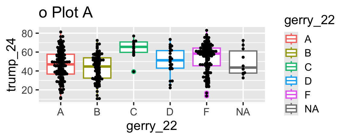
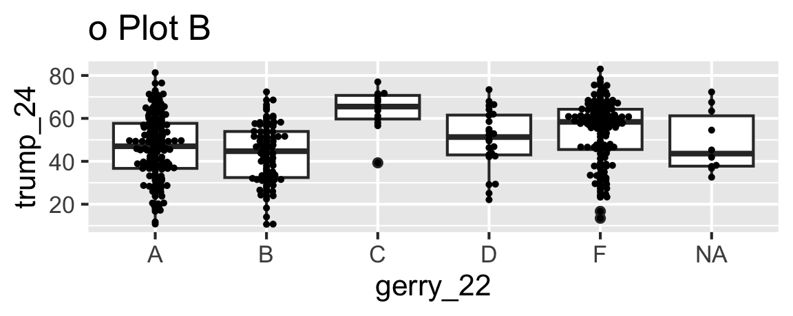
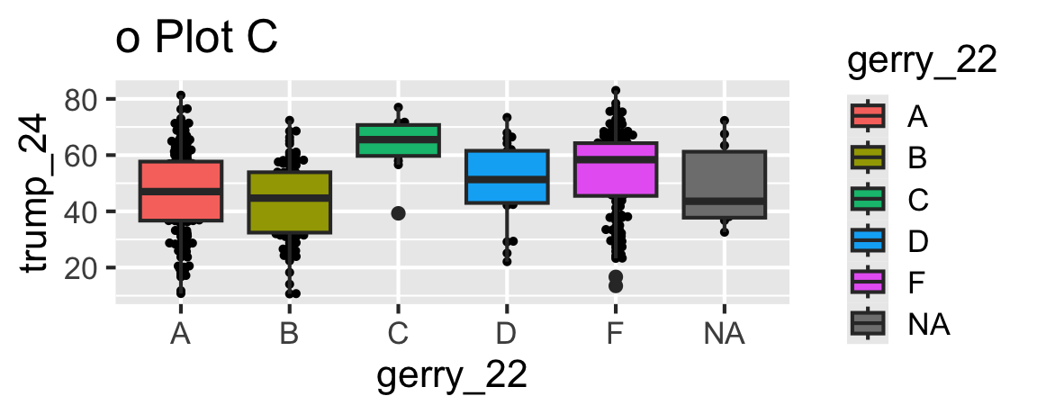
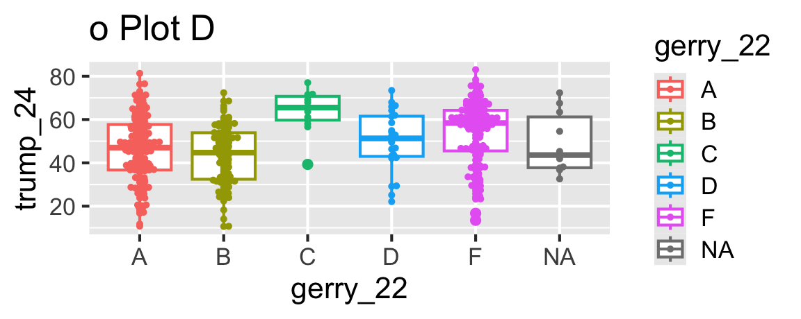
Go to wooclap.com and use the code ICNGKSL.

Pause

Any questions before we get started?

Recap: layering geoms

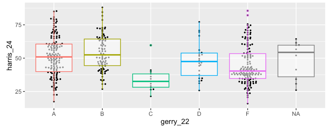
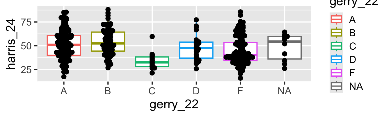
Update the following code to create the visualization on the right.

ggplot(gerrymander_24, aes(x = gerry_22, y = harris_24)) +
  geom_boxplot(aes(color = gerry_22)) +
  geom_beeswarm()

Recap: layering geoms

Original Code:

ggplot(gerrymander_24, aes(x = gerry_22, y = harris_24)) +
  geom_boxplot(aes(color = gerry_22)) +
  geom_beeswarm()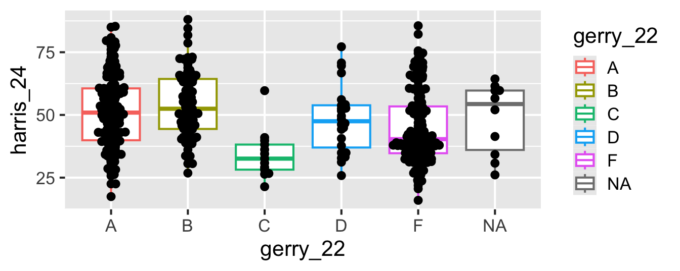

Recap: layering geoms

Swap the order of the two geoms.

ggplot(gerrymander_24, aes(x = gerry_22, y = harris_24)) +
  geom_beeswarm(size = 0.8) +
  geom_boxplot(aes(color = gerry_22))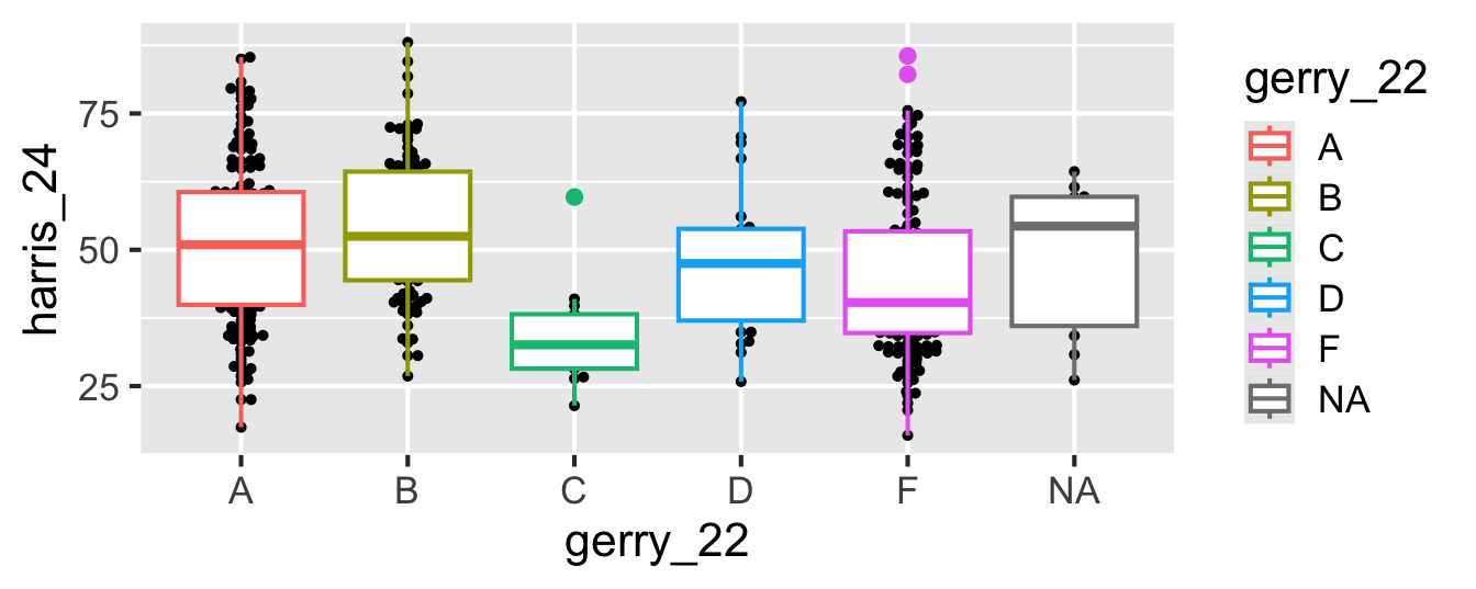

Recap: layering geoms

Make the boxplots semi-transparent.

ggplot(gerrymander_24, aes(x = gerry_22, y = harris_24)) +
  geom_beeswarm(size = 0.8) +
  geom_boxplot(aes(color = gerry_22), alpha = 0.5)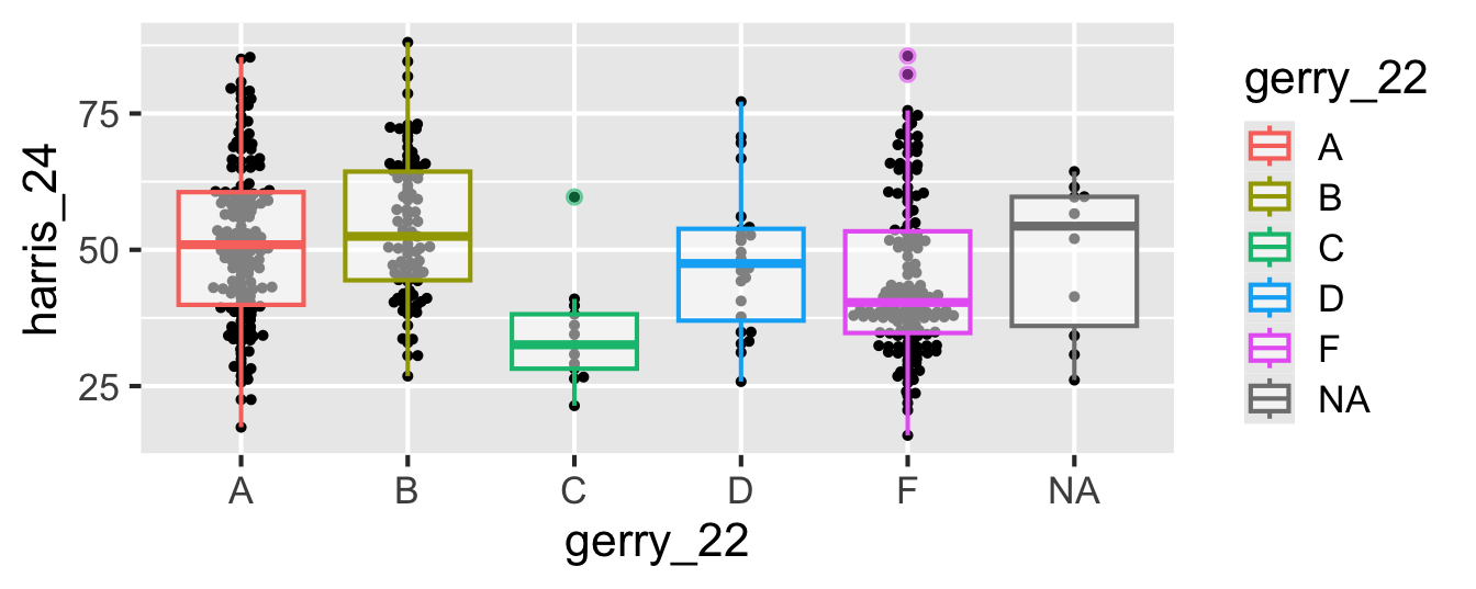

Recap: layering geoms

Remove the legend.

ggplot(gerrymander_24, aes(x = gerry_22, y = harris_24)) +
  geom_beeswarm(size = 0.8) +
  geom_boxplot(aes(color = gerry_22), alpha = 0.5, show.legend = FALSE)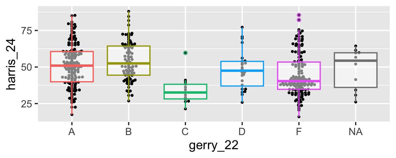

Recap: logical operators

Generally useful in a filter() but will come up in various other places as well…

operator	definition
`<`	is less than?
`>`	is greater than?

Recap: Participate 📱💻

Match the following logical operators to their definitions.

<=
>=
==
!=

Go to wooclap.com and use the code ICNGKSL.

Recap: Participate 📱💻

Match the following definitions to their logical operators.

is x AND y?
is x OR y?
is x NA?
is x not NA?

Go to wooclap.com and use the code ICNGKSL.

Recap: logical operators (cont.)

Other useful logical operators:

operator	definition
`x %in% y`	is x in y?
`!(x %in% y)`	is x not in y?
`!x`	is not x? (only makes sense if `x` is `TRUE` or `FALSE`)

Recap: logical operators (cont.)

For which rows are the following true?

Col1	Col2	Col3
1	A	50
2	B	40
3	A	30
4	B	NA
5	C	10

Col1 < 3 | Col3 < 20
Col2 == "C"
Col2 %in% c("C", "A")
is.na(Col3)
!is.na(Col3)

Data tidying

Tidy data

“Tidy datasets are easy to manipulate, model and visualise, and have a specific structure: each variable is a column, each observation is a row, and each type of observational unit is a table.”

Tidy Data, https://vita.had.co.nz/papers/tidy-data.pdf

Note: “easy to manipulate” = “straightforward to manipulate”

Goal

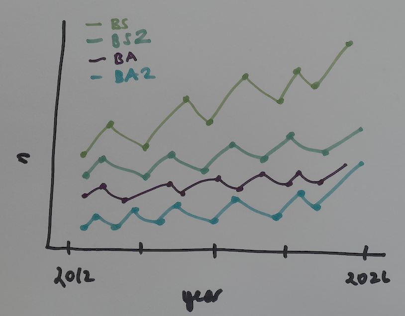
Visualize Statistical Science majors over the years!

Read data

majors <- read_csv("data/majors.csv")

Rows: 33 Columns: 17
── Column specification ────────────────────────────────────────────────────────
Delimiter: ","
chr  (2): department, academic_plan
dbl (15): 2026, 2025, 2024, 2023, 2022, 2021, 2020, 2019, 2018, 2017, 2016, ...

ℹ Use `spec()` to retrieve the full column specification for this data.
ℹ Specify the column types or set `show_col_types = FALSE` to quiet this message.

What does the message that prints when we read a CSV file in with read_csv() say? How carefully do you need to review this message before moving on?

View data

majors

# A tibble: 33 × 17
   department     academic_plan `2026` `2025` `2024` `2023` `2022` `2021` `2020`
   <chr>          <chr>          <dbl>  <dbl>  <dbl>  <dbl>  <dbl>  <dbl>  <dbl>
 1 Biology        BS               151    151    147    146    141    159    147
 2 Biology        BS2               13     13     11     11      5     11      4
 3 Biology        BA                10      5     11     11      6      6      8
 4 Biology        BA2                1      4      2      1      8      1      3
 5 Biology        Minor             54     59     51     65     70     68     50
 6 Computer Scie… BS               238    209    247    213    190    187    170
 7 Computer Scie… BS2              150    125    105     76     43     38     33
 8 Computer Scie… BA                24     29     27     36     20     32     45
 9 Computer Scie… BA2               44     30     43     34     27     32     21
10 Computer Scie… Minor             53     78     72     75     62     58     57
# ℹ 23 more rows
# ℹ 8 more variables: `2019` <dbl>, `2018` <dbl>, `2017` <dbl>, `2016` <dbl>,
#   `2015` <dbl>, `2014` <dbl>, `2013` <dbl>, `2012` <dbl>

Data dictionary

Variable	Description
`department`	Academic department offering the major or minor.
`academic_plan`	BS: Bachelor of Science; BS2: Bachelor of Science, second major; BA: Bachelor of Arts; BA2: Bachelor of Arts, second major; Minor: a minor in the department.
`2026`:`2012`	Each column gives the number of graduates completing that academic plan in the corresponding academic year. `NA` indicates no count recorded.

What does each row in majors represent?

Each row represents a department and academic plan combination.

Let’s plan!

Review the goal plot and sketch the data frame needed to create it. What would go inside aes when we call ggplot?

First: `filter()`

statsci_majors <- majors |>
  filter(
    department == "Statistical Science",
    academic_plan != "Minor"
  )

statsci_majors

# A tibble: 4 × 17
  department      academic_plan `2026` `2025` `2024` `2023` `2022` `2021` `2020`
  <chr>           <chr>          <dbl>  <dbl>  <dbl>  <dbl>  <dbl>  <dbl>  <dbl>
1 Statistical Sc… BS                49     45     39     54     32     35     27
2 Statistical Sc… BS2               28     23     20     27     16     17     17
3 Statistical Sc… BA                 2     NA      1      2     NA     NA      1
4 Statistical Sc… BA2                1     NA     NA     NA     NA      2      1
# ℹ 8 more variables: `2019` <dbl>, `2018` <dbl>, `2017` <dbl>, `2016` <dbl>,
#   `2015` <dbl>, `2014` <dbl>, `2013` <dbl>, `2012` <dbl>

The Goal

We want to write code that starts something like this:

ggplot(statsci_majors, aes(x = year, y = n, color = academic_plan)) +
  ...

But the data are not organized in the appropriate columns :(

statsci_majors

# A tibble: 4 × 17
  department      academic_plan `2026` `2025` `2024` `2023` `2022` `2021` `2020`
  <chr>           <chr>          <dbl>  <dbl>  <dbl>  <dbl>  <dbl>  <dbl>  <dbl>
1 Statistical Sc… BS                49     45     39     54     32     35     27
2 Statistical Sc… BS2               28     23     20     27     16     17     17
3 Statistical Sc… BA                 2     NA      1      2     NA     NA      1
4 Statistical Sc… BA2                1     NA     NA     NA     NA      2      1
# ℹ 8 more variables: `2019` <dbl>, `2018` <dbl>, `2017` <dbl>, `2016` <dbl>,
#   `2015` <dbl>, `2014` <dbl>, `2013` <dbl>, `2012` <dbl>

The challenge

How do we go from this ….

# A tibble: 4 × 17
  department      academic_plan `2026` `2025` `2024` `2023` `2022` `2021` `2020`
  <chr>           <chr>          <dbl>  <dbl>  <dbl>  <dbl>  <dbl>  <dbl>  <dbl>
1 Statistical Sc… BS                49     45     39     54     32     35     27
2 Statistical Sc… BS2               28     23     20     27     16     17     17
3 Statistical Sc… BA                 2     NA      1      2     NA     NA      1
4 Statistical Sc… BA2                1     NA     NA     NA     NA      2      1
# ℹ 8 more variables: `2019` <dbl>, `2018` <dbl>, `2017` <dbl>, `2016` <dbl>,
#   `2015` <dbl>, `2014` <dbl>, `2013` <dbl>, `2012` <dbl>

…. to this??

# A tibble: 60 × 4
   department          academic_plan  year     n
   <chr>               <chr>         <dbl> <dbl>
 1 Statistical Science BS             2026    49
 2 Statistical Science BS             2025    45
 3 Statistical Science BS             2024    39
 4 Statistical Science BS             2023    54
 5 Statistical Science BS             2022    32
 6 Statistical Science BS             2021    35
 7 Statistical Science BS             2020    27
 8 Statistical Science BS             2019    26
 9 Statistical Science BS             2018    21
10 Statistical Science BS             2017    24
# ℹ 50 more rows

Pivot

`pivot_longer()`

# A tibble: 4 × 17
  department      academic_plan `2026` `2025` `2024` `2023` `2022` `2021` `2020`
  <chr>           <chr>          <dbl>  <dbl>  <dbl>  <dbl>  <dbl>  <dbl>  <dbl>
1 Statistical Sc… BS                49     45     39     54     32     35     27
2 Statistical Sc… BS2               28     23     20     27     16     17     17
3 Statistical Sc… BA                 2     NA      1      2     NA     NA      1
4 Statistical Sc… BA2                1     NA     NA     NA     NA      2      1
# ℹ 8 more variables: `2019` <dbl>, `2018` <dbl>, `2017` <dbl>, `2016` <dbl>,
#   `2015` <dbl>, `2014` <dbl>, `2013` <dbl>, `2012` <dbl>

⬇️

Pivot the statsci_majors data frame longer such that each row represents a degree type / year combination. The new columns should be called year and n (for number of graduates for that year).

# A tibble: 60 × 4
   department          academic_plan  year     n
   <chr>               <chr>         <dbl> <dbl>
 1 Statistical Science BS             2026    49
 2 Statistical Science BS             2025    45
 3 Statistical Science BS             2024    39
 4 Statistical Science BS             2023    54
 5 Statistical Science BS             2022    32
 6 Statistical Science BS             2021    35
 7 Statistical Science BS             2020    27
 8 Statistical Science BS             2019    26
 9 Statistical Science BS             2018    21
10 Statistical Science BS             2017    24
# ℹ 50 more rows

`pivot_longer()`

# A tibble: 4 × 17
  department      academic_plan `2026` `2025` `2024` `2023` `2022` `2021` `2020`
  <chr>           <chr>          <dbl>  <dbl>  <dbl>  <dbl>  <dbl>  <dbl>  <dbl>
1 Statistical Sc… BS                49     45     39     54     32     35     27
2 Statistical Sc… BS2               28     23     20     27     16     17     17
3 Statistical Sc… BA                 2     NA      1      2     NA     NA      1
4 Statistical Sc… BA2                1     NA     NA     NA     NA      2      1
# ℹ 8 more variables: `2019` <dbl>, `2018` <dbl>, `2017` <dbl>, `2016` <dbl>,
#   `2015` <dbl>, `2014` <dbl>, `2013` <dbl>, `2012` <dbl>

⬇️

statsci_majors |>
  pivot_longer(
    cols = ___________________,

    names_to = _______________,

    values_to = ______________
  )

# A tibble: 60 × 4
   department          academic_plan  year     n
   <chr>               <chr>         <dbl> <dbl>
 1 Statistical Science BS             2026    49
 2 Statistical Science BS             2025    45
 3 Statistical Science BS             2024    39
 4 Statistical Science BS             2023    54
 5 Statistical Science BS             2022    32
 6 Statistical Science BS             2021    35
 7 Statistical Science BS             2020    27
 8 Statistical Science BS             2019    26
 9 Statistical Science BS             2018    21
10 Statistical Science BS             2017    24
# ℹ 50 more rows

`pivot_longer()`

What goes in each of the blanks?

statsci_majors |>
  pivot_longer(
    cols = ___________________, # columns to pivot

    names_to = _______________, # what the new variable name should be

    values_to = ______________  # where the new variable name should come from
  )

How did it go?

We started with:

# A tibble: 4 × 17
  department      academic_plan `2026` `2025` `2024` `2023` `2022` `2021` `2020`
  <chr>           <chr>          <dbl>  <dbl>  <dbl>  <dbl>  <dbl>  <dbl>  <dbl>
1 Statistical Sc… BS                49     45     39     54     32     35     27
2 Statistical Sc… BS2               28     23     20     27     16     17     17
3 Statistical Sc… BA                 2     NA      1      2     NA     NA      1
4 Statistical Sc… BA2                1     NA     NA     NA     NA      2      1
# ℹ 8 more variables: `2019` <dbl>, `2018` <dbl>, `2017` <dbl>, `2016` <dbl>,
#   `2015` <dbl>, `2014` <dbl>, `2013` <dbl>, `2012` <dbl>

⬇️ Then we pivoted

We wanted:

# A tibble: 60 × 4
   department          academic_plan  year     n
   <chr>               <chr>         <dbl> <dbl>
 1 Statistical Science BS             2026    49
 2 Statistical Science BS             2025    45
 3 Statistical Science BS             2024    39
 4 Statistical Science BS             2023    54
 5 Statistical Science BS             2022    32
 6 Statistical Science BS             2021    35
 7 Statistical Science BS             2020    27
 8 Statistical Science BS             2019    26
 9 Statistical Science BS             2018    21
10 Statistical Science BS             2017    24
# ℹ 50 more rows

But we got:

# A tibble: 60 × 4
   department          academic_plan year      n
   <chr>               <chr>         <chr> <dbl>
 1 Statistical Science BS            2026     49
 2 Statistical Science BS            2025     45
 3 Statistical Science BS            2024     39
 4 Statistical Science BS            2023     54
 5 Statistical Science BS            2022     32
 6 Statistical Science BS            2021     35
 7 Statistical Science BS            2020     27
 8 Statistical Science BS            2019     26
 9 Statistical Science BS            2018     21
10 Statistical Science BS            2017     24
# ℹ 50 more rows

Can you spot the difference?

`year`

What is the type of the year variable? Why? What should it be?

statsci_majors |>
  pivot_longer(
    cols = !c(department, academic_plan),
    values_to = "n",
    names_to = "year"
  )

# A tibble: 60 × 4
   department          academic_plan year      n
   <chr>               <chr>         <chr> <dbl>
 1 Statistical Science BS            2026     49
 2 Statistical Science BS            2025     45
 3 Statistical Science BS            2024     39
 4 Statistical Science BS            2023     54
 5 Statistical Science BS            2022     32
 6 Statistical Science BS            2021     35
 7 Statistical Science BS            2020     27
 8 Statistical Science BS            2019     26
 9 Statistical Science BS            2018     21
10 Statistical Science BS            2017     24
# ℹ 50 more rows

It’s a character (chr) variable since the information came from the column names of the original data frame.
R cannot know that these character strings represent years.
We need to tell R that the variable type of year should be numeric.

`pivot_longer()` again

Let’s pivot again, this time making sure also that year is a numerical variable in the resulting data frame.

statsci_majors |>
  pivot_longer(
    cols = !c(department, academic_plan),
    values_to = "n",
    names_to = "year",
    names_transform = as.numeric
  )

# A tibble: 60 × 4
   department          academic_plan  year     n
   <chr>               <chr>         <dbl> <dbl>
 1 Statistical Science BS             2026    49
 2 Statistical Science BS             2025    45
 3 Statistical Science BS             2024    39
 4 Statistical Science BS             2023    54
 5 Statistical Science BS             2022    32
 6 Statistical Science BS             2021    35
 7 Statistical Science BS             2020    27
 8 Statistical Science BS             2019    26
 9 Statistical Science BS             2018    21
10 Statistical Science BS             2017    24
# ℹ 50 more rows

Application exercise

Goal: Make this plot

`ae-03: StatSci majors`

Go to your ae project in Positron.
If you haven’t yet done so, make sure all of your changes up to this point are committed and pushed, i.e., there’s nothing left in your source control pane.
Pull to get today’s application exercise file: ae-03-statsci-majors.qmd.
Work through the application exercise in class, and render, commit, and push your edits by the end of class.

Pivot wider

We pivotted longer… what about wider?

# A tibble: 4 × 17
  department      academic_plan `2026` `2025` `2024` `2023` `2022` `2021` `2020`
  <chr>           <chr>          <dbl>  <dbl>  <dbl>  <dbl>  <dbl>  <dbl>  <dbl>
1 Statistical Sc… BS                49     45     39     54     32     35     27
2 Statistical Sc… BS2               28     23     20     27     16     17     17
3 Statistical Sc… BA                 2     NA      1      2     NA     NA      1
4 Statistical Sc… BA2                1     NA     NA     NA     NA      2      1
# ℹ 8 more variables: `2019` <dbl>, `2018` <dbl>, `2017` <dbl>, `2016` <dbl>,
#   `2015` <dbl>, `2014` <dbl>, `2013` <dbl>, `2012` <dbl>

⬆️

Can we go the other direction?

# A tibble: 60 × 4
   department          academic_plan  year     n
   <chr>               <chr>         <dbl> <dbl>
 1 Statistical Science BS             2026    49
 2 Statistical Science BS             2025    45
 3 Statistical Science BS             2024    39
 4 Statistical Science BS             2023    54
 5 Statistical Science BS             2022    32
 6 Statistical Science BS             2021    35
 7 Statistical Science BS             2020    27
 8 Statistical Science BS             2019    26
 9 Statistical Science BS             2018    21
10 Statistical Science BS             2017    24
# ℹ 50 more rows

We pivotted longer… what about wider?

# A tibble: 4 × 17
  department      academic_plan `2026` `2025` `2024` `2023` `2022` `2021` `2020`
  <chr>           <chr>          <dbl>  <dbl>  <dbl>  <dbl>  <dbl>  <dbl>  <dbl>
1 Statistical Sc… BS                49     45     39     54     32     35     27
2 Statistical Sc… BS2               28     23     20     27     16     17     17
3 Statistical Sc… BA                 2     NA      1      2     NA     NA      1
4 Statistical Sc… BA2                1     NA     NA     NA     NA      2      1
# ℹ 8 more variables: `2019` <dbl>, `2018` <dbl>, `2017` <dbl>, `2016` <dbl>,
#   `2015` <dbl>, `2014` <dbl>, `2013` <dbl>, `2012` <dbl>

⬆️

statsci_majors_longer |>
  pivot_wider(
    names_from = _______,

    values_from = ______________
  )

# A tibble: 60 × 4
   department          academic_plan  year     n
   <chr>               <chr>         <dbl> <dbl>
 1 Statistical Science BS             2026    49
 2 Statistical Science BS             2025    45
 3 Statistical Science BS             2024    39
 4 Statistical Science BS             2023    54
 5 Statistical Science BS             2022    32
 6 Statistical Science BS             2021    35
 7 Statistical Science BS             2020    27
 8 Statistical Science BS             2019    26
 9 Statistical Science BS             2018    21
10 Statistical Science BS             2017    24
# ℹ 50 more rows

`pivot_wider()`

statsci_majors_longer |>
  pivot_wider(
    names_from = year,
    values_from = n
  )

# A tibble: 4 × 17
  department      academic_plan `2026` `2025` `2024` `2023` `2022` `2021` `2020`
  <chr>           <chr>          <dbl>  <dbl>  <dbl>  <dbl>  <dbl>  <dbl>  <dbl>
1 Statistical Sc… BS                49     45     39     54     32     35     27
2 Statistical Sc… BS2               28     23     20     27     16     17     17
3 Statistical Sc… BA                 2     NA      1      2     NA     NA      1
4 Statistical Sc… BA2                1     NA     NA     NA     NA      2      1
# ℹ 8 more variables: `2019` <dbl>, `2018` <dbl>, `2017` <dbl>, `2016` <dbl>,
#   `2015` <dbl>, `2014` <dbl>, `2013` <dbl>, `2012` <dbl>

Recap: Pivoting

When should you pivot? If all of the data you need is in your data frame, but the data are not organized in the columns you need, there is a good chance you need to pivot!
Wide and long: Data sets can’t be labeled as wide or long but they can be made wider or longer for a certain analysis that requires a certain shape.
Pivot longer - data type: When pivoting longer, variable names that turn into values are characters by default. If you need them to be in another format, you need to explicitly make that transformation, which you can do so within the pivot_longer() function.

Recap: Plotting

You can tweak a plot forever, but at some point the tweaks are likely not very productive.
However, you should always be critical of defaultsand see if you can improve the plot to better portray your data / results / what you want to communicate.

Tidying data

Warm-up

While you wait: Participate 📱💻

Pause

Recap: layering geoms

Recap: layering geoms

Recap: layering geoms

Recap: layering geoms

Recap: layering geoms

Recap: logical operators

Recap: Participate 📱💻

Recap: Participate 📱💻

Recap: logical operators (cont.)

Recap: logical operators (cont.)

Data tidying

Tidy data

Goal

Read data

View data

Data dictionary

Let’s plan!

First: filter()

The Goal

The challenge

Pivot

pivot_longer()

pivot_longer()

pivot_longer()

How did it go?

year

pivot_longer() again

Application exercise

Goal: Make this plot

ae-03: StatSci majors

Pivot wider

We pivotted longer… what about wider?

We pivotted longer… what about wider?

pivot_wider()

Recap: Pivoting

Recap: Plotting

First: `filter()`

`pivot_longer()`

`pivot_longer()`

`pivot_longer()`

`year`

`pivot_longer()` again

`ae-03: StatSci majors`

`pivot_wider()`