Joining data

Lecture 8

Dr. Mine Çetinkaya-Rundel

Duke University
STA 199 - Fall 2026

September 21, 2026

Warm-up

While you wait: Participate 📱💻

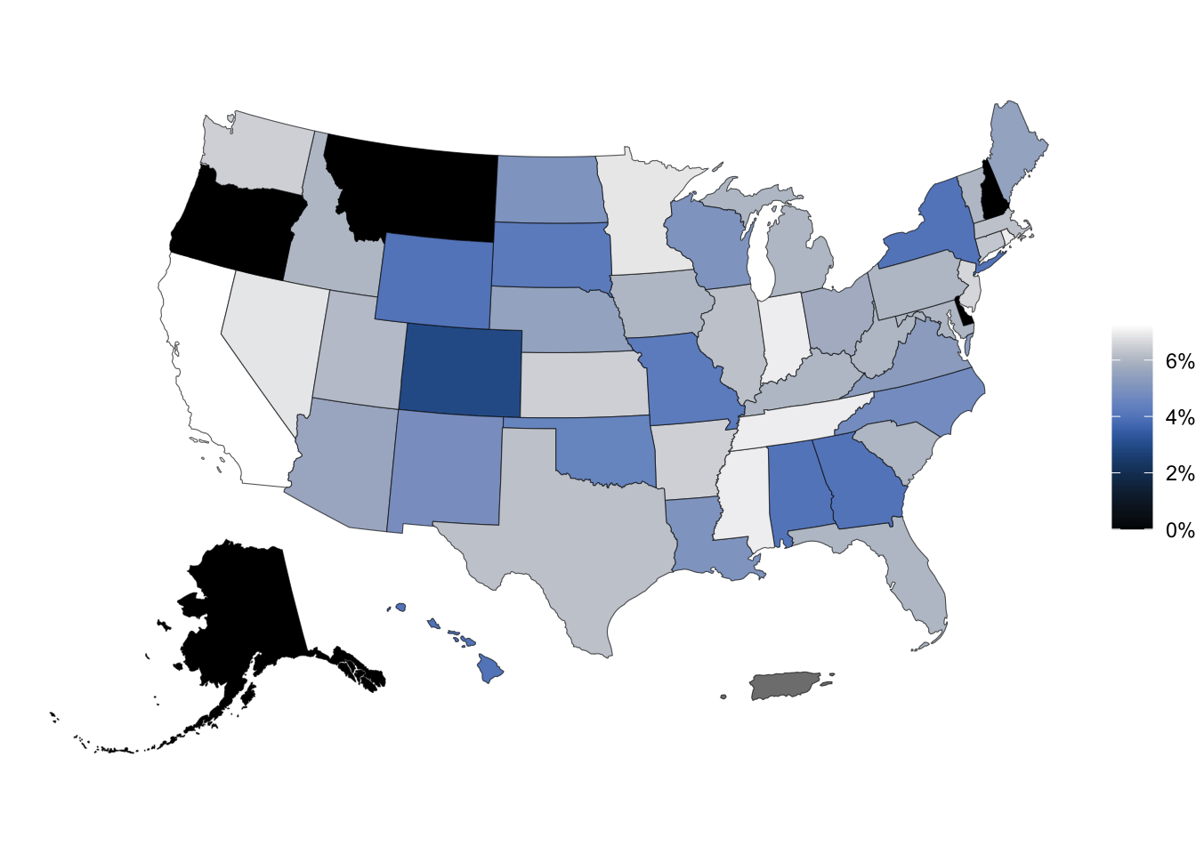
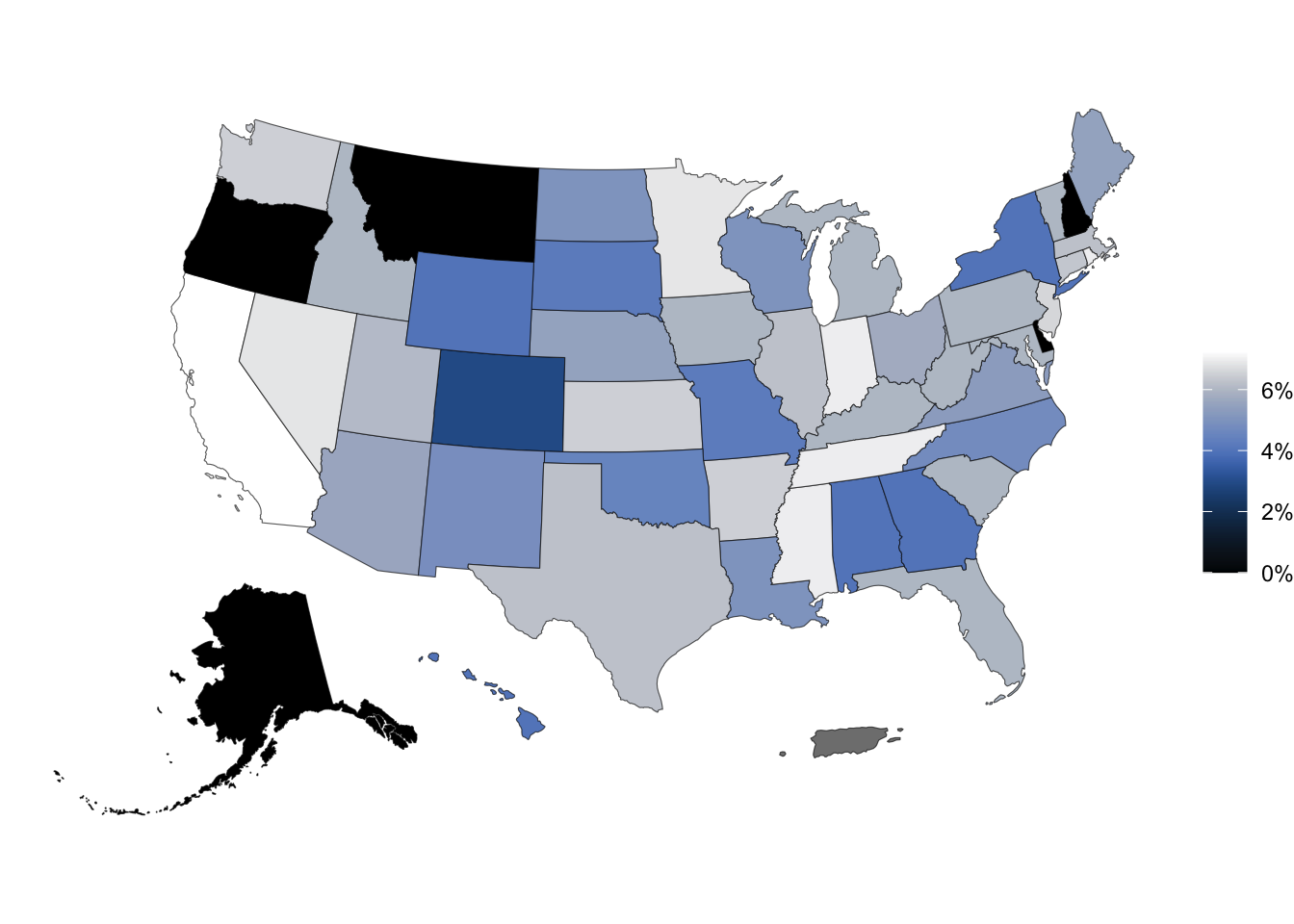
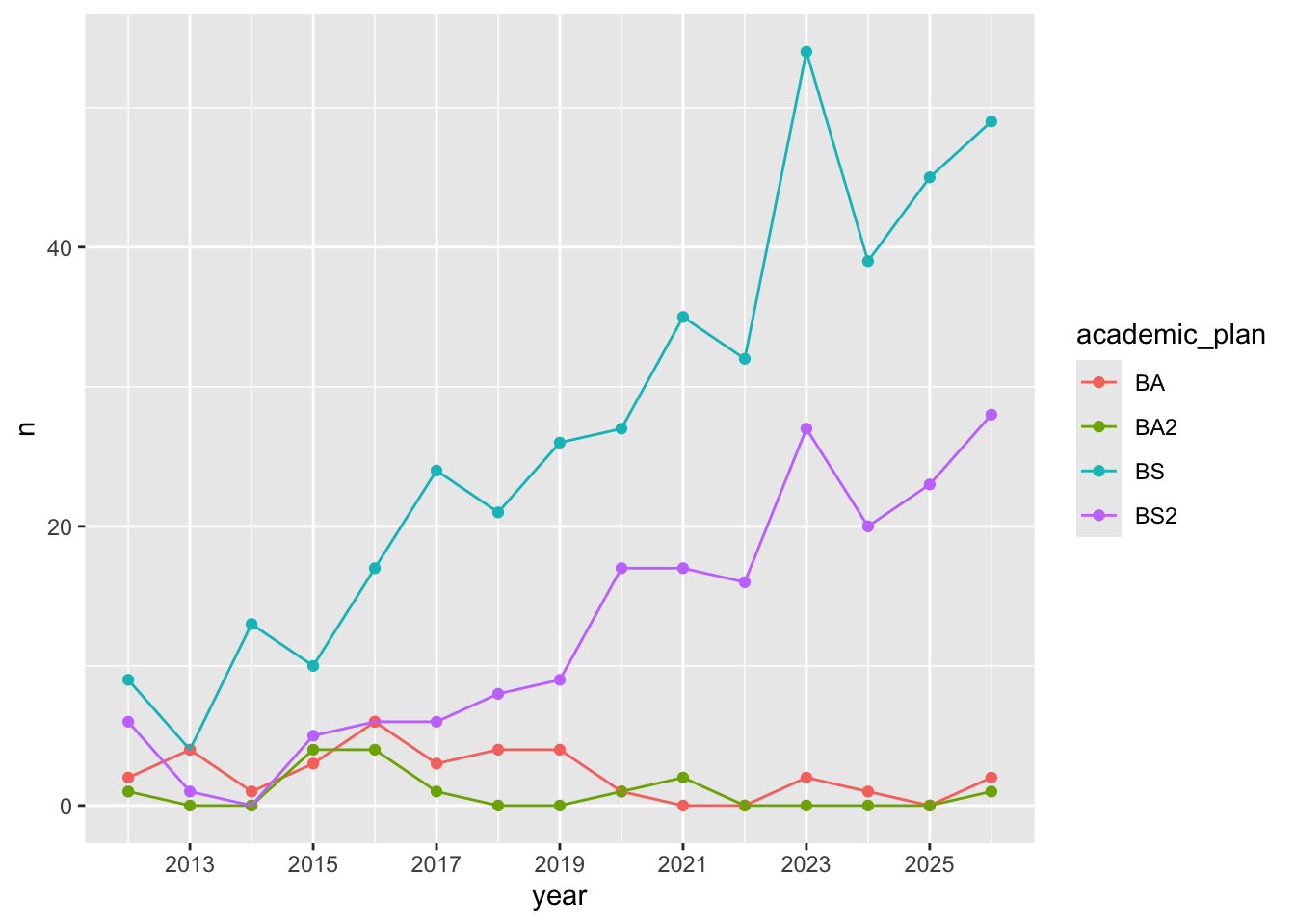
Can you guess the variable plotted here?

Go to wooclap.com and use the code PYDPUEI.

Announcements

If you have received an email from Dr. Knox about missing labs, HWs, commits, files on GitHub or Gradescope:
- Step 1: Don’t panic – these emails are just to make sure you don’t repeatedly make the same errors throughout assignments
- Step 2:
  - If you’re not sure how to address the issues, please write back ASAP so we can help you!
  - If you know how to address it, make sure to do so in your following assignment!

If you’ve enjoyed working with classmates in your randomly assigned labs so far and/or if you have identified common interests, reach out to them to see if you might form a project team together. You’ll get a chance to share these preferences in lab on Thursday.

Recap: from last AE

Any questions about how we left off last time to where AE-03 goes by the end? Or where to find the AE answers?

Where we left off:

Where the AE-03 ends:

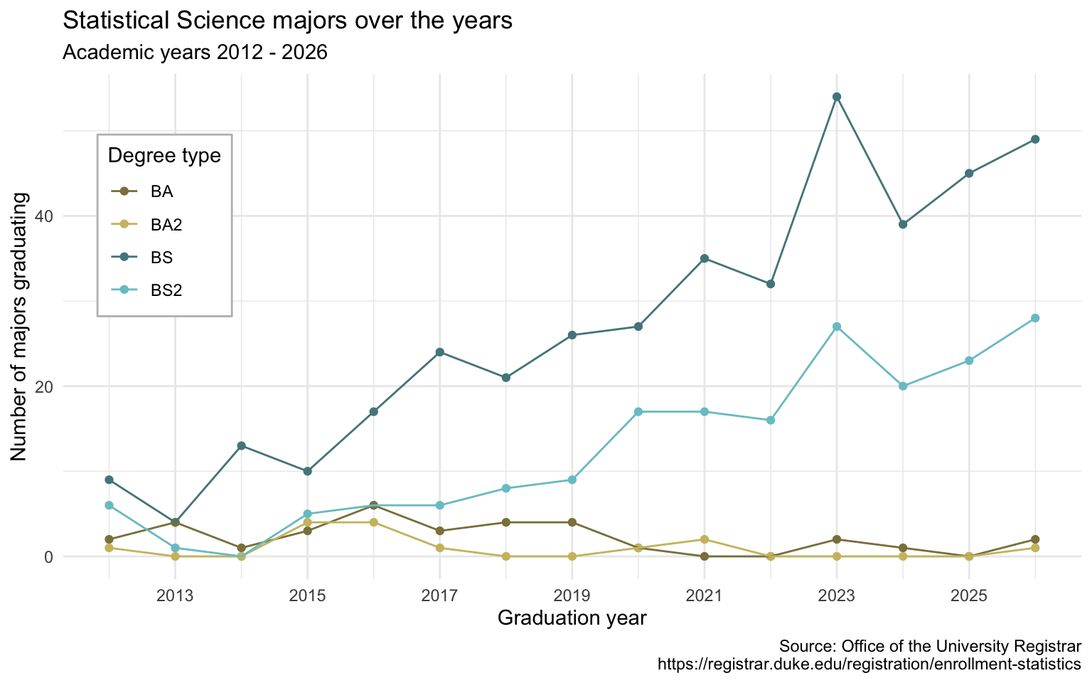
Recoding data

Let’s look at the results…

Sales taxes in US states

sales_taxes

# A tibble: 51 × 7
   state       state_tax_rate state_tax_rank avg_local_tax_rate max_local
   <chr>                <dbl>          <dbl>              <dbl>     <dbl>
 1 Alabama               4                40               5.46     11   
 2 Alaska                0                46               1.82      7.85
 3 Arizona               5.6              28               2.92      5.3 
 4 Arkansas              6.5               9               2.96      6.12
 5 California            7.25              1               1.74      5.25
 6 Colorado              2.9              45               4.99      9.1 
 7 Connecticut           6.35             12               0         0   
 8 Delaware              0                46               0         0   
 9 Florida               6                17               0.98      2   
10 Georgia               4                40               3.49      5   
# ℹ 41 more rows
# ℹ 2 more variables: combined_tax_rate <dbl>, combined_rank <dbl>

Participate 📱💻

Put the following steps in order to compare the average state sales tax rates of swing states (Arizona, Georgia, Michigan, Nevada, North Carolina, Pennsylvania, and Wisconsin) vs. non-swing states:

Group by swing_state
Summarize to find the mean sales tax in each type of state
Create a new variable called swing_state with levels "Swing" and "Non-swing"

Go to wooclap.com and use the code PYDPUEI.

Participate 📱💻

First, create a vector called list_of_swing_states that contains the names of the swing states.

list_of_swing_states <- c(
  "Arizona", "Georgia", "Michigan", "Nevada", "North Carolina",
  "Pennsylvania", "Wisconsin"
)

Then, fill in the blanks to create a new variable called swing_state with levels "Swing" and "Non-swing":

sales_taxes <- sales_taxes |>
  __BLANK_1__(
    swing_state = __BLANK_2__(
      state __BLANK_3__ list_of_swing_states, "Swing", "Non-swing"
    )
  )

Go to wooclap.com and use the code PYDPUEI.

Recap: `if_else()`

if_else(
1  x == y,
2  "x is equal to y",
3  "x is not equal to y"
)

1: Condition
2: Value if condition is TRUE
3: Value if condition is FALSE

Participate 📱💻

Fill in the blank to compare the average state sales tax rates of swing states vs. non-swing states.

sales_taxes |>
  __BLANK__ |>
  summarize(mean_state_tax = mean(state_tax_rate))

arrange(swing_state)
filter(swing_state == "Swing")
group_by(swing_state)
group_by(list_of_swing_states)

Go to wooclap.com and use the code PYDPUEI.

Sales tax in swing states

sales_taxes |>
  group_by(swing_state) |>
  summarize(mean_state_tax = mean(state_tax_rate))

# A tibble: 2 × 2
  swing_state mean_state_tax
  <chr>                <dbl>
1 Non-swing             5.05
2 Swing                 5.46

Sales tax in coastal states

Suppose you’re tasked with the following:

Compare the average state sales tax rates of states on the Pacific Coast, states on the Atlantic Coast, and the rest of the states.

How would you approach this task?

Create a new variable called coast with levels "Pacific", "Atlantic", and "Neither"
Group by coast
Summarize to find the mean sales tax in each type of state

Participate 📱💻

First, create two vectors called pacific_coast and atlantic_coast that contain the respective states.

pacific_coast <- c("Alaska", "Washington", "Oregon", "California", "Hawaii")

atlantic_coast <- c(
  "Connecticut", "Delaware", "Georgia", "Florida", "Maine", "Maryland", 
  "Massachusetts", "New Hampshire", "New Jersey", "New York", 
  "North Carolina", "Rhode Island", "South Carolina", "Virginia"
)

Then, fill in the blank to create a new variable called coast:

sales_taxes <- sales_taxes |>
  mutate(
    coast = __BLANK__(
      state %in% atlantic_coast ~ "Atlantic",
      state %in% pacific_coast ~ "Pacific",
      .default = "Neither"
    )
  )

Go to wooclap.com and use the code PYDPUEI.

Recap: `case_when()`

case_when(
1  x > y ~ "x is greater than y",
2  x < y ~ "x is less than y",
3  .default = "x is equal to y"
)

1: Value if first condition is TRUE
2: Value if second condition is TRUE
3: Value if neither condition is TRUE, i.e., default value

Sales tax in coastal states

Compare the average state sales tax rates of states on the Pacific Coast, states on the Atlantic Coast, and the rest of the states.

sales_taxes |>
  group_by(coast) |>
  summarize(mean_state_tax = mean(state_tax_rate))

# A tibble: 3 × 2
  coast    mean_state_tax
  <chr>             <dbl>
1 Atlantic           4.84
2 Neither            5.46
3 Pacific            3.55

Sales tax in US regions

Suppose you’re tasked with the following:

Compare the average state sales tax rates of states in various regions (Midwest - 12 states, Northeast - 9 states, South - 16 states, West - 13 states).

How would you approach this task?

Create a new variable called region with levels "Midwest", "Northeast", "South", and "West".
Group by region
Summarize to find the mean sales tax in each type of state

`mutate()` with `case_when()`

Who feels like filling in the blanks lists of states in each region? Who feels like it’s simply too tedious to write out names of all states?

list_of_midwest_states <- c(___)
list_of_northeast_states <- c(___)
list_of_south_states <- c(___)
list_of_west_states <- c(___)

sales_taxes <- sales_taxes |>
  mutate(
    region = case_when(
      state %in% list_of_midwest_states ~ "Midwest",
      state %in% list_of_northeast_states ~ "Northeast",
      state %in% list_of_south_states ~ "South",
      state %in% list_of_west_states ~ "West"
    )
  )

Joining data

Why join?

Suppose we want to answer questions like:

Is there a relationship between
- number of QS courses taken
- having scored a 4 or 5 on the AP stats exam
- motivation for taking course
- …
and performance in this course?

Each of these would require joining class performance data with an outside data source so we can have all relevant information (columns) in a single data frame.

Why join?

Suppose we want to answer questions like:

Compare the average state sales tax rates of states in various regions (Midwest - 12 states, Northeast - 9 states, South - 16 states, West - 13 states).

This can also be solved with joining region information with the state-level sales tax data.

Setup

For the next few slides…

x <- tibble(
  id = c(1, 2, 3),
  value_x = c("x1", "x2", "x3")
)

x

# A tibble: 3 × 2
     id value_x
  <dbl> <chr>  
1     1 x1     
2     2 x2     
3     3 x3

y <- tibble(
  id = c(1, 2, 4),
  value_y = c("y1", "y2", "y4")
)

y

# A tibble: 3 × 2
     id value_y
  <dbl> <chr>  
1     1 y1     
2     2 y2     
3     4 y4

`left_join()`

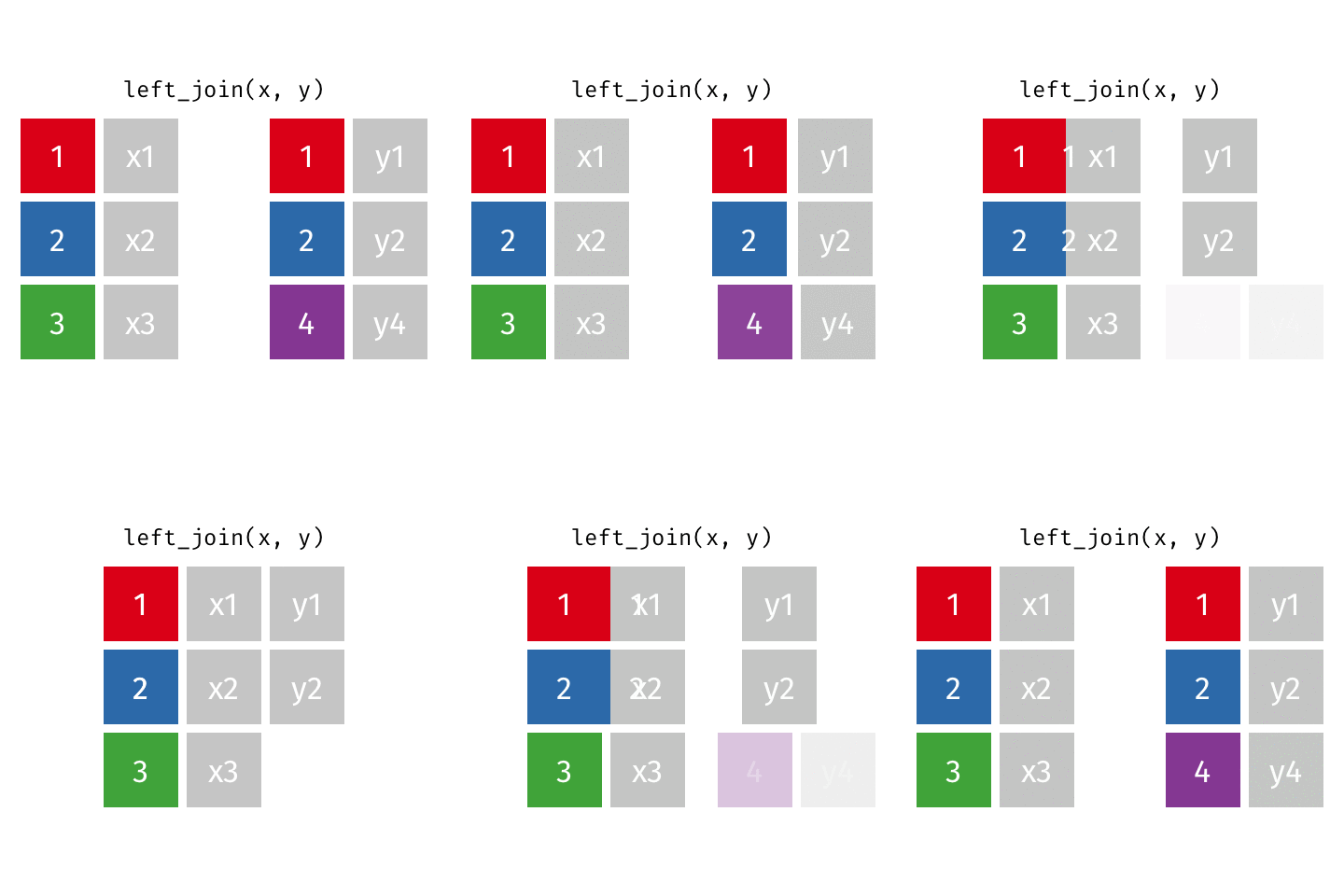
left_join(x, y)

Joining with `by = join_by(id)`

# A tibble: 3 × 3
     id value_x value_y
  <dbl> <chr>   <chr>  
1     1 x1      y1     
2     2 x2      y2     
3     3 x3      <NA>

`right_join()`

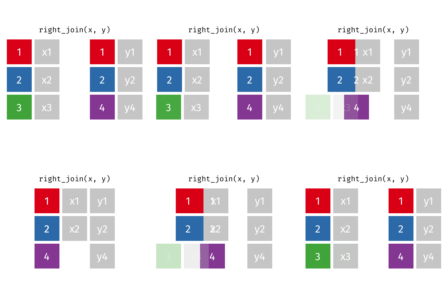
right_join(x, y)

Joining with `by = join_by(id)`

# A tibble: 3 × 3
     id value_x value_y
  <dbl> <chr>   <chr>  
1     1 x1      y1     
2     2 x2      y2     
3     4 <NA>    y4

`full_join()`

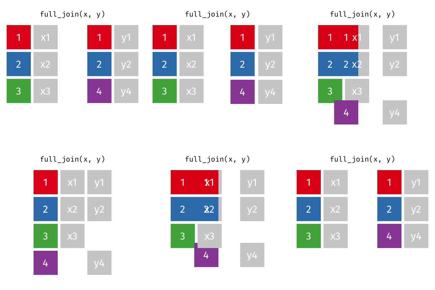
full_join(x, y)

Joining with `by = join_by(id)`

# A tibble: 4 × 3
     id value_x value_y
  <dbl> <chr>   <chr>  
1     1 x1      y1     
2     2 x2      y2     
3     3 x3      <NA>   
4     4 <NA>    y4

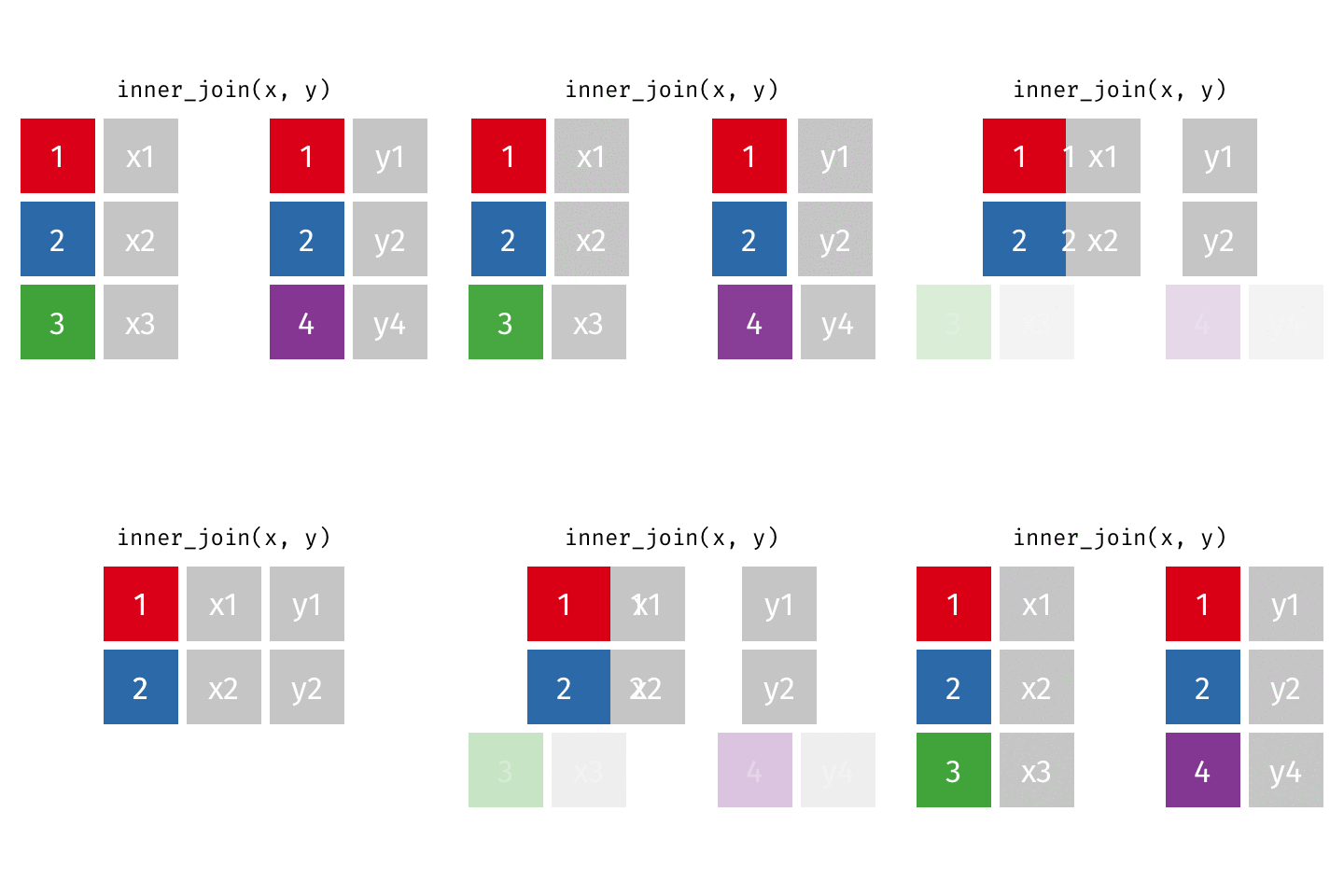
`inner_join()`

inner_join(x, y)

Joining with `by = join_by(id)`

# A tibble: 2 × 3
     id value_x value_y
  <dbl> <chr>   <chr>  
1     1 x1      y1     
2     2 x2      y2

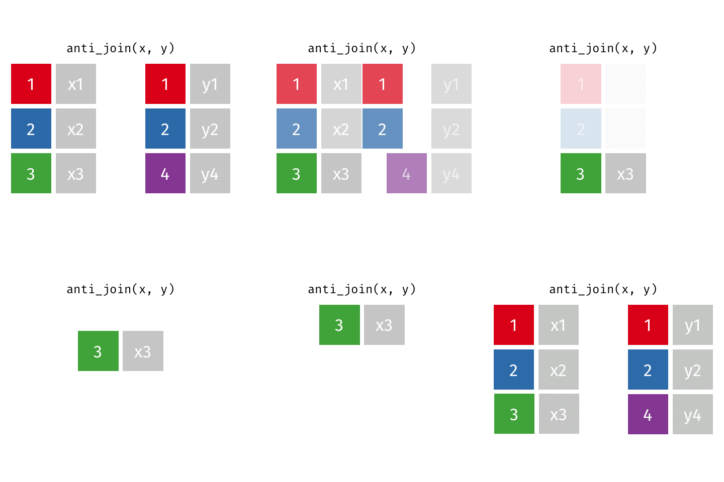
`anti_join()`

anti_join(x, y)

Joining with `by = join_by(id)`

# A tibble: 1 × 2
     id value_x
  <dbl> <chr>  
1     3 x3

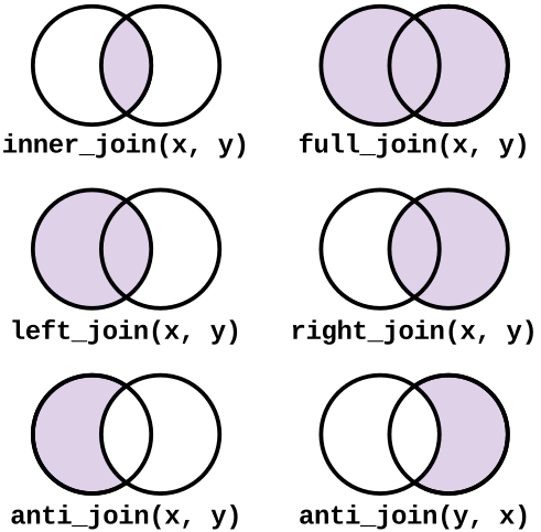
Summary of joins

Application exercise

Goal

Compare the average state sales tax rates of states in various regions (Midwest, Northeast, South, West), where the input data are:

States and sales taxes: sales-taxes-26.csv
States and regions: us-regions.csv

`ae-04-taxes-join`

Go to your ae project in Positron.
If you haven’t yet done so, make sure all of your changes up to this point are committed and pushed, i.e., there’s nothing left in your source control pane.
If you haven’t yet done so, pull to get today’s application exercise file: ae-04-taxes-join.qmd.
Work through the application exercise in class, and render, commit, and push your edits by the end of class.

Joining data

Warm-up

While you wait: Participate 📱💻

Announcements

Recap: from last AE

Recoding data

Let’s look at the results…

Sales taxes in US states

Participate 📱💻

Participate 📱💻

Recap: if_else()

Participate 📱💻

Sales tax in swing states

Sales tax in coastal states

Participate 📱💻

Recap: case_when()

Sales tax in coastal states

Sales tax in US regions

mutate() with case_when()

Joining data

Why join?

Why join?

Setup

left_join()

right_join()

full_join()

inner_join()

anti_join()

Summary of joins

Application exercise

Goal

ae-04-taxes-join

Recap: `if_else()`

Recap: `case_when()`

`mutate()` with `case_when()`

`left_join()`

`right_join()`

`full_join()`

`inner_join()`

`anti_join()`

`ae-04-taxes-join`