Lecture 15
Duke University
STA 199 - Fall 2026
October 21, 2026
What questions could a model help us answer about community health?

Go to wooclap.com and use the code BSAFXJG.
By the end of today, you should be able to:
Prediction: Use known information to estimate an unknown outcome.
Description / explanation: Summarize how an outcome tends to vary with a predictor.
What questions could a model help us answer about community health?
PLACES: Local Data for Better Health is a free CDC resource providing consistently defined health and health-related estimates for communities across the US.
Important
These are model-based local estimates, not direct survey estimates for each county.
The CDC PLACES 2025 release provides local health estimates for every U.S. county.
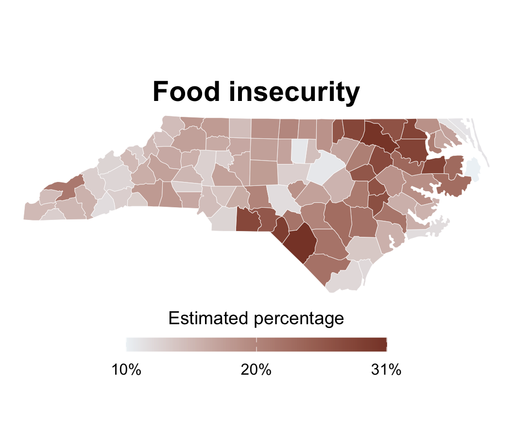
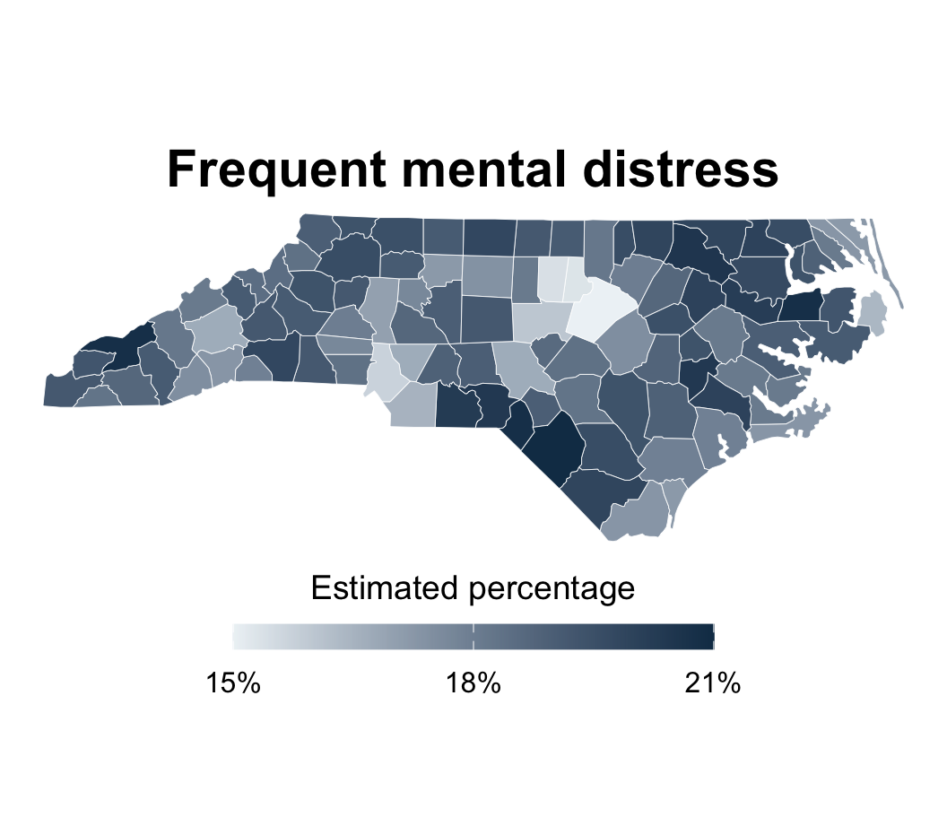
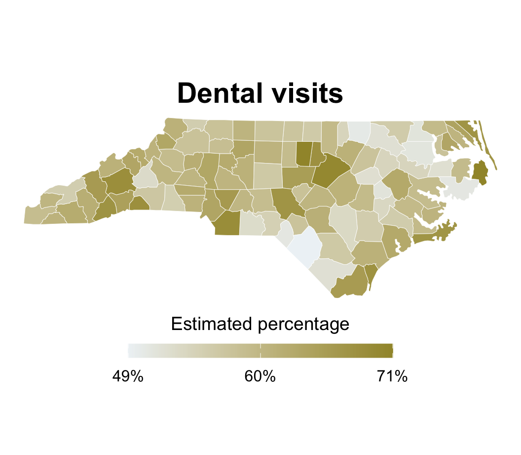
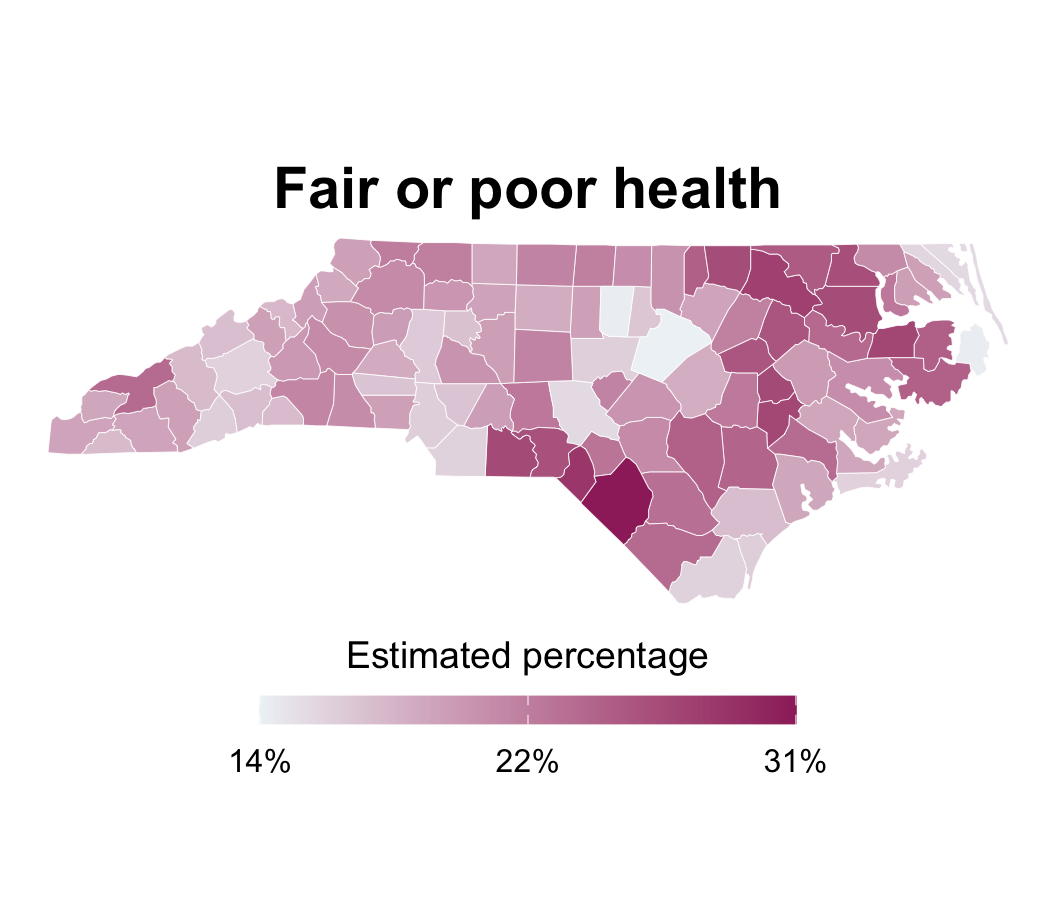
For North Carolina, we will explore:
Both are age-adjusted, model-based estimates derived from 2023 survey and population data.
NC Department of Commerce county tiers: The 40 most distressed counties are designated as Tier 1, the next 40 as Tier 2 and the 20 least distressed as Tier 3
NC Office of State Archaeology regions: Piedmont, Mountains, Coastal Plain
nc-places.csv.tidyverse for data wrangling and visualization
scales for better axis labels
tidymodels for modeling with tidyverse principles
maps for county boundaries
Rows: 100 Columns: 46
ββ Column specification ββββββββββββββββββββββββββββββββββββββββββββββββββββββββ
Delimiter: ","
chr (4): county, development_tier, region, appalachian
dbl (42): county_fips, food_insecurity, mental_distress, dental_visit, fair_...
βΉ Use `spec()` to retrieve the full column specification for this data.
βΉ Specify the column types or set `show_col_types = FALSE` to quiet this message.
food_insecurity - Food insecurity: % of adults who experienced food insecurity during the previous 12 months.mental_distress - Frequent mental distress: % of adults who experienced at least 14 mentally unhealthy days during the previous 30 days.

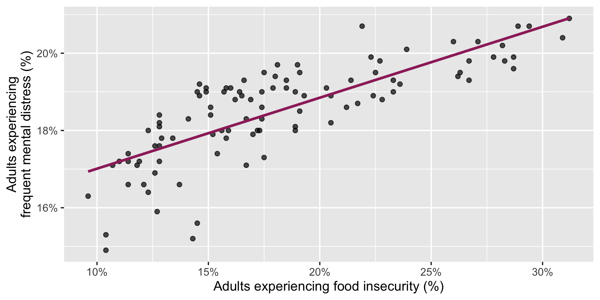
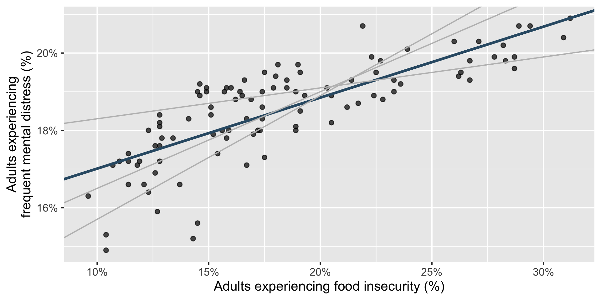
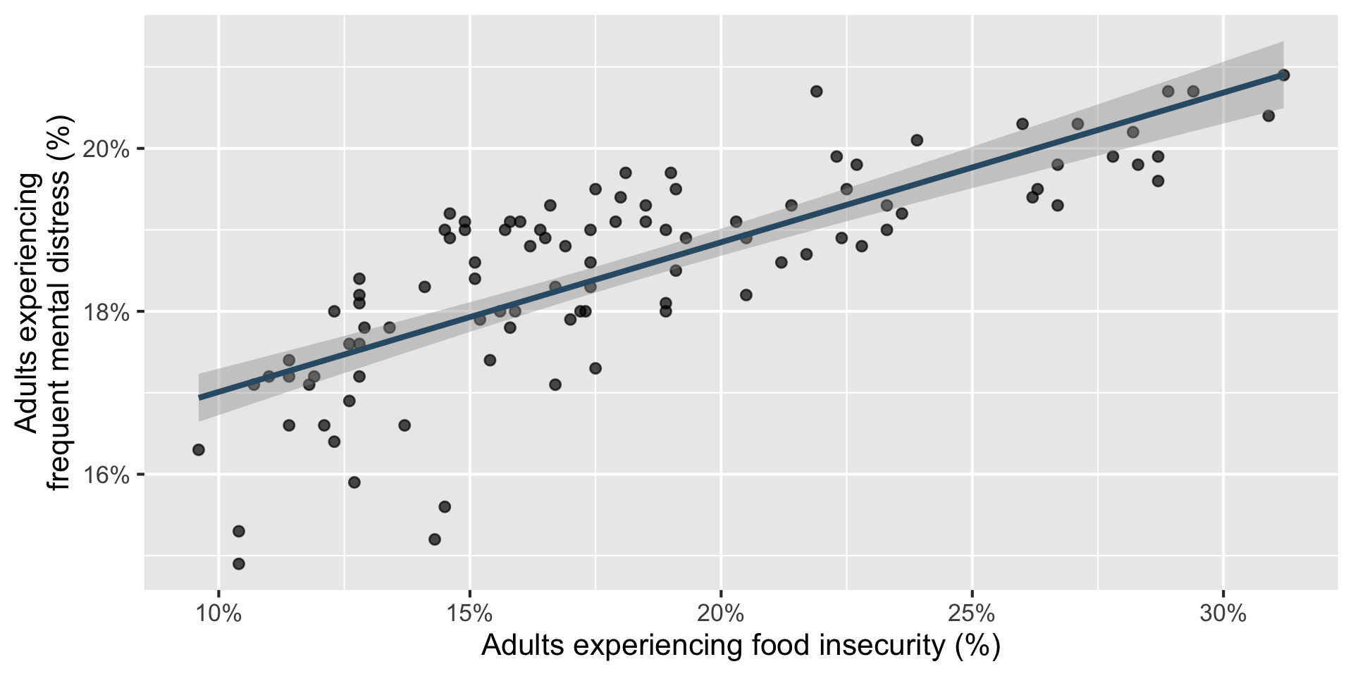
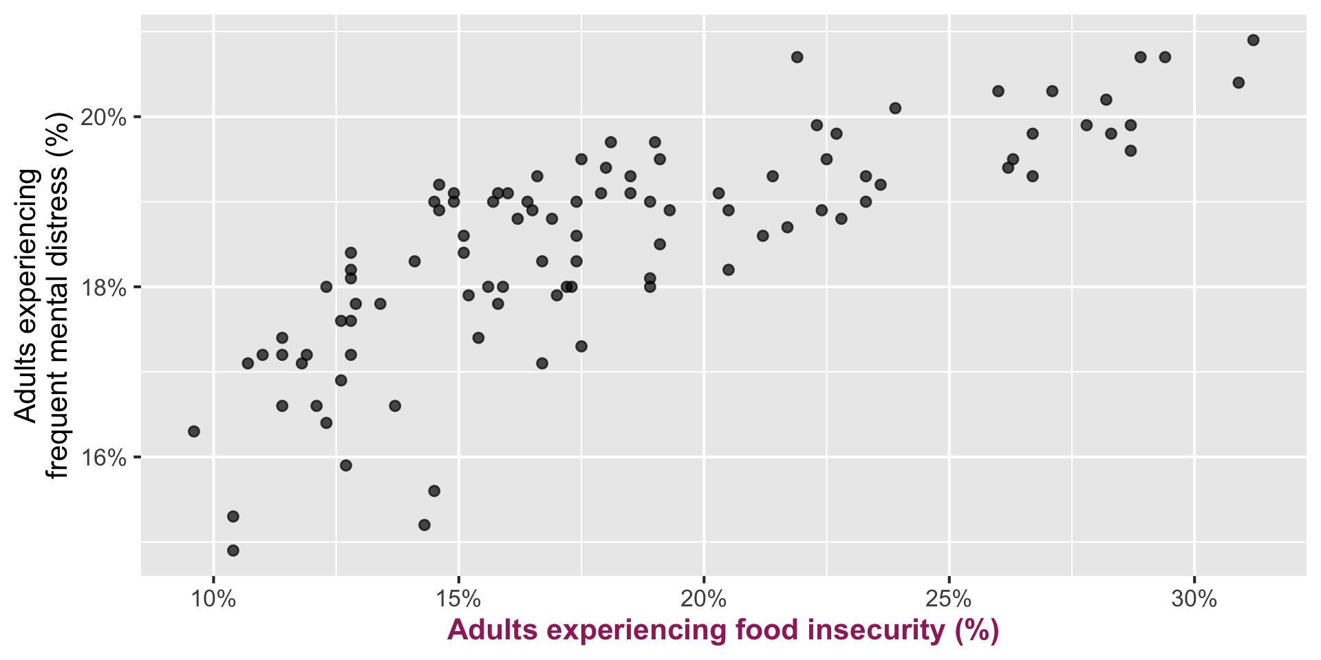
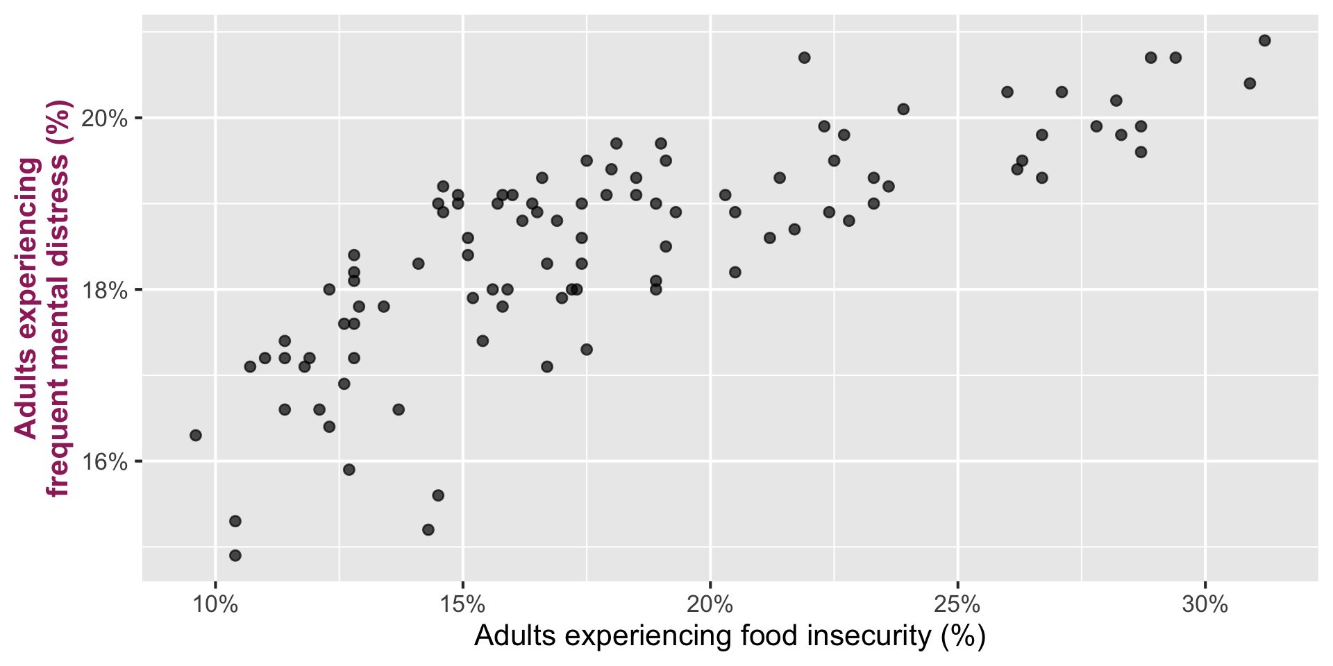
Describe: How is county-level food insecurity related to frequent mental distress?
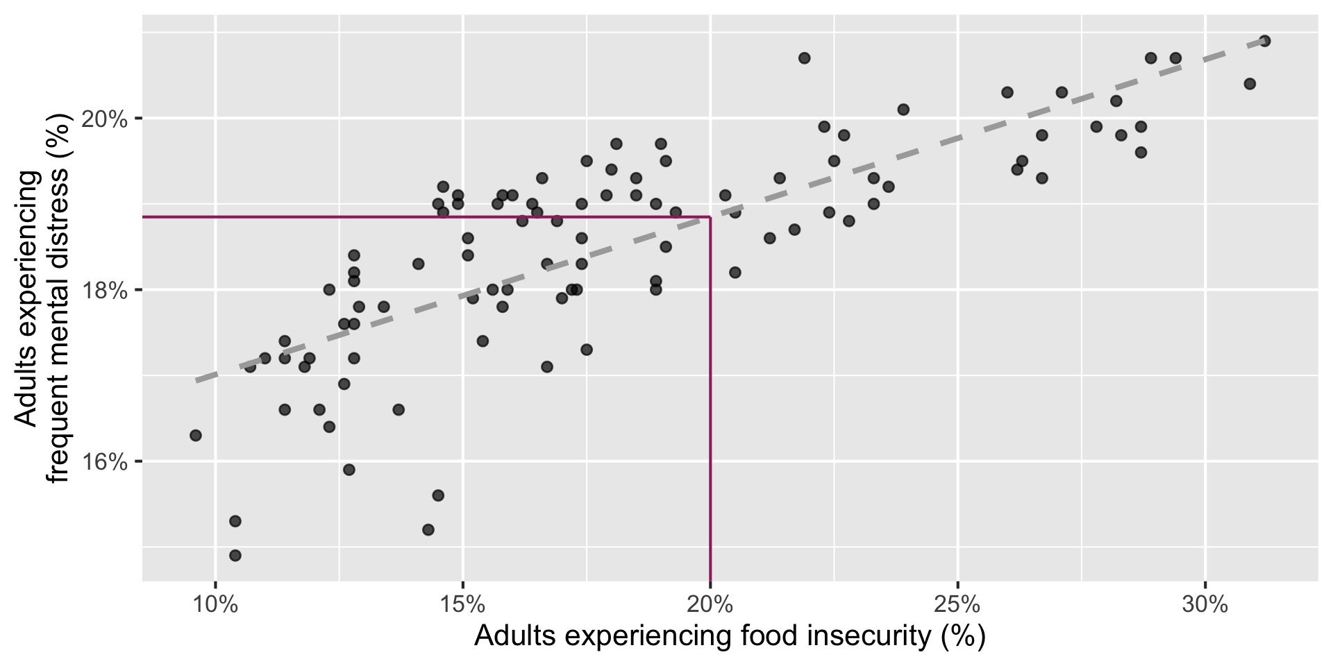
Predict: For a county where 20% of adults experience food insecurity, what percentage would we predict experience frequent mental distress?
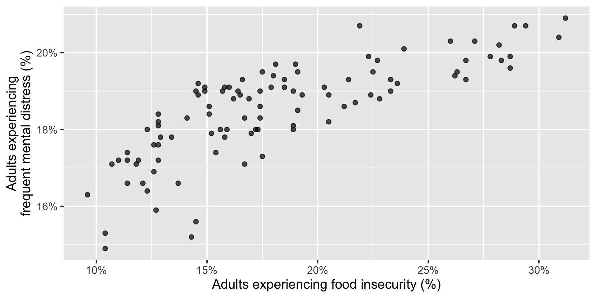
Describe: How is county-level food insecurity related to frequent mental distress?
Predict: For a county where 20% of adults experience food insecurity, what percentage would we predict experience frequent mental distress?
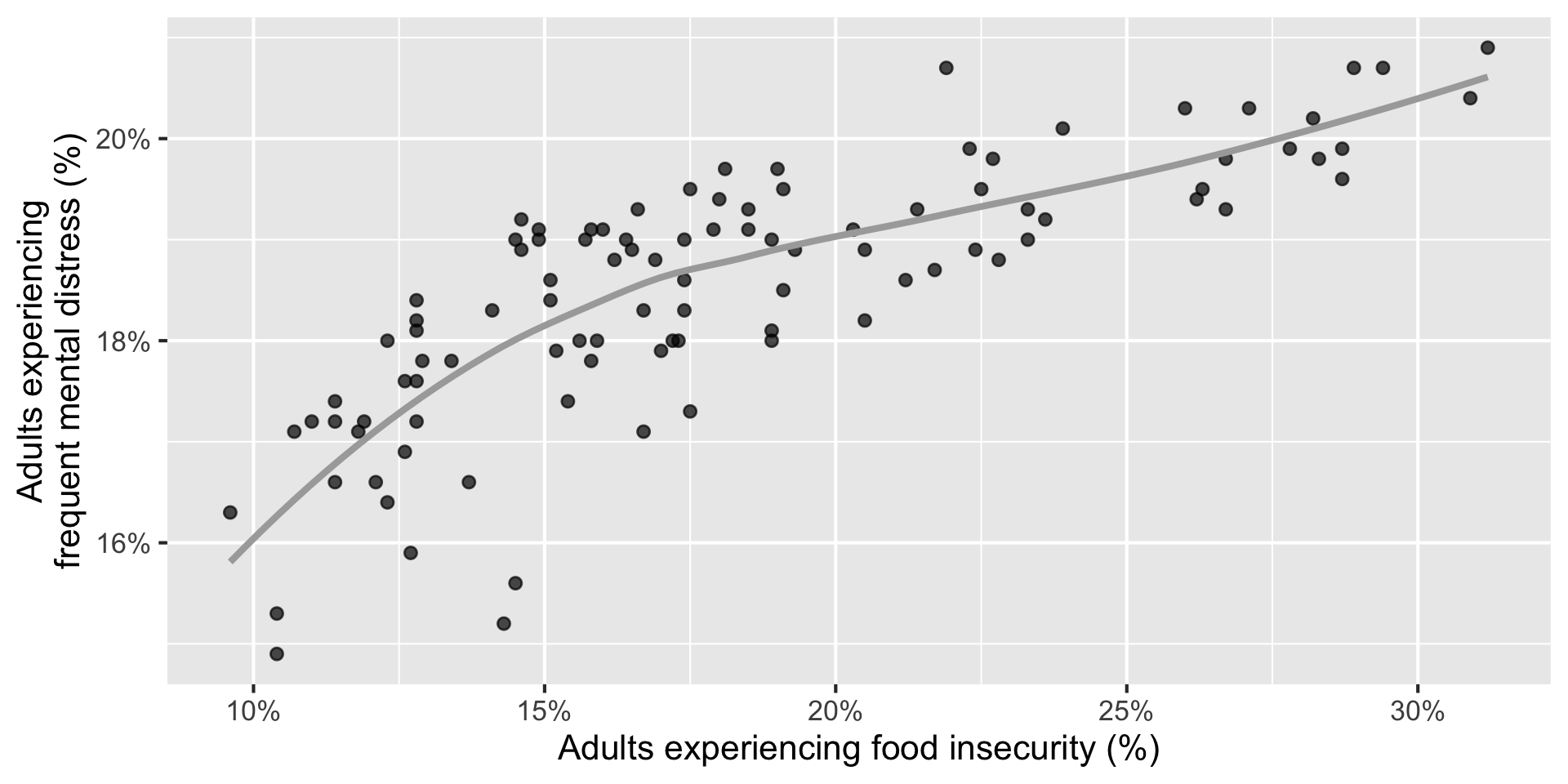
Use models to describe relationships between variables and to make predictions.
For now, we will focus on linear modelsβbut there are many other types of models.
| county | food_insecurity | mental_distress |
|---|---|---|
| Alamance | 17.2 | 18 |
| Alexander | 15.8 | 19.1 |
| Alleghany | 18.5 | 19.3 |
| Anson | 28.2 | 20.2 |
| Ashe | 14.6 | 18.9 |
| Avery | 15.1 | 18.4 |
| ... | ... | ... |
| county | food_insecurity | mental_distress |
|---|---|---|
| Alamance | 17.2 | 18 |
| Alexander | 15.8 | 19.1 |
| Alleghany | 18.5 | 19.3 |
| Anson | 28.2 | 20.2 |
| Ashe | 14.6 | 18.9 |
| Avery | 15.1 | 18.4 |
| ... | ... | ... |
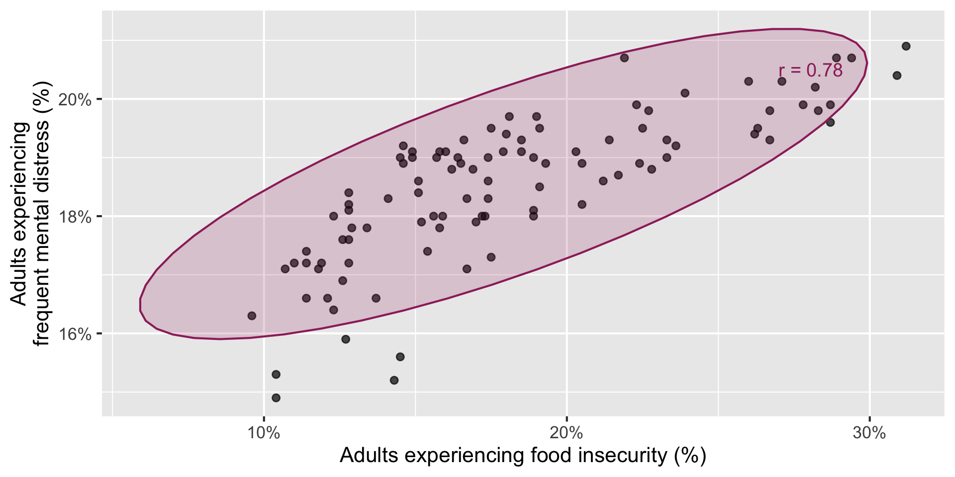
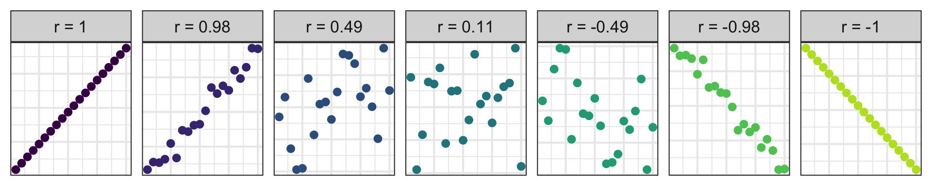
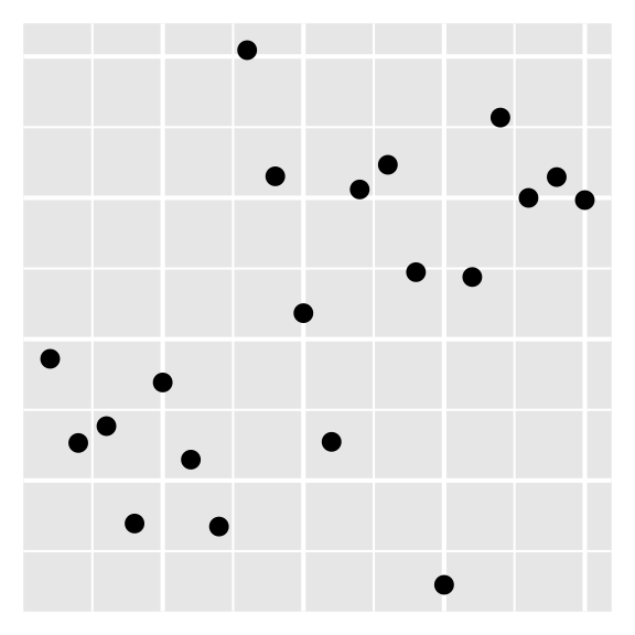
Which of the following is the best guess for the correlation between the two variables below?

Go to wooclap.com and use the code BSAFXJG.
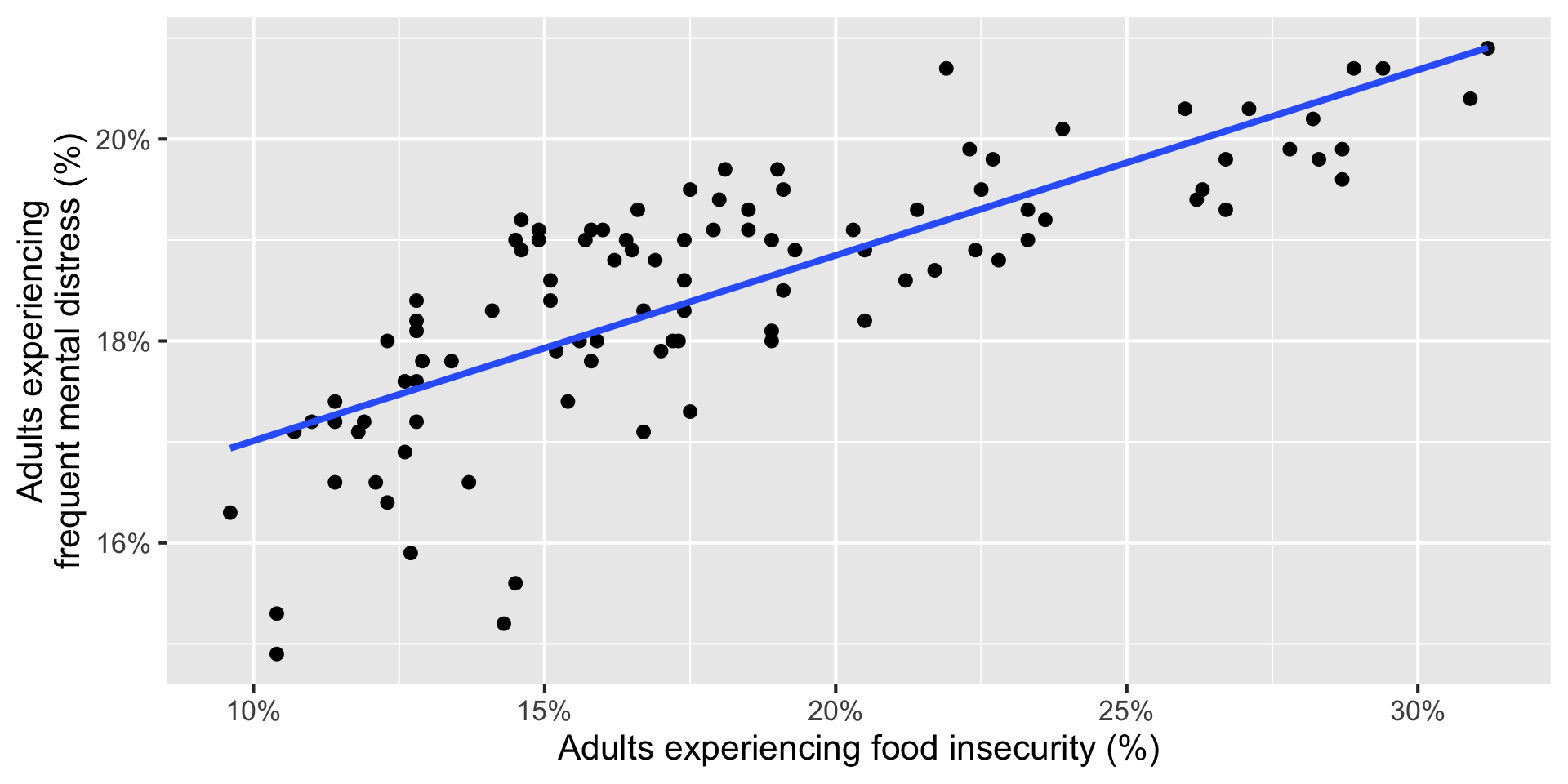
ggplot(
nc_places,
aes(x = food_insecurity, y = mental_distress)
) +
geom_point() +
geom_smooth(method = "lm", se = FALSE) +
scale_x_continuous(labels = percent_label()) +
scale_y_continuous(labels = percent_label()) +
labs(
x = "Adults experiencing food insecurity (%)",
y = "Adults experiencing\nfrequent mental distress (%)"
)A regression model separates an observed outcome into a systematic part and an unexplained part:
\[ \begin{aligned} Y &= \text{Model} + \text{Error} \\ &= f(X) + \epsilon \\ &= \mu_{Y \mid X} + \epsilon \end{aligned} \]
A linear regression model describes the relationship between a quantitative outcome, \(Y\), and a quantitative predictor, \(X\):
\[ Y = \beta_0 + \beta_1 X + \epsilon \]
We use data to estimate the population relationship:
\[ \widehat{Y} = b_0 + b_1 X \]
Note
There is no error term in the fitted line: \(\widehat{Y}\) is the modelβs prediction, not an observed outcome.
Using mathematical notation
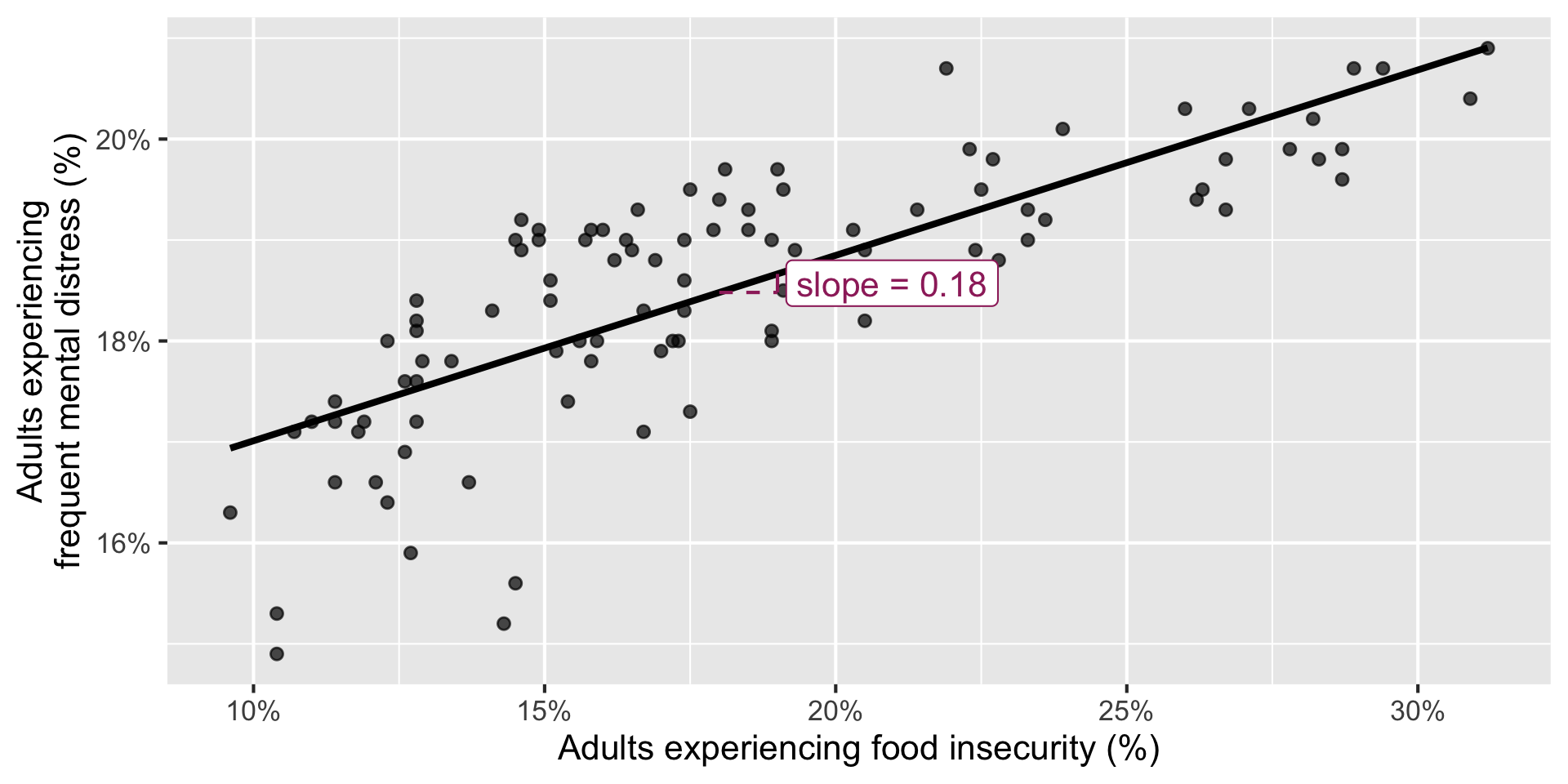
\[ \widehat{\text{mental distress %}} = 15.2 + 0.184 \times \text{food insecurity %} \]
Reading the model equation
Predicted mental-distress percentage is 15.2 plus 0.184 times the food insecurity percentage.
The slope of the fitted model is 0.184. Which of the following is the best interpretation?

Go to wooclap.com and use the code BSAFXJG.
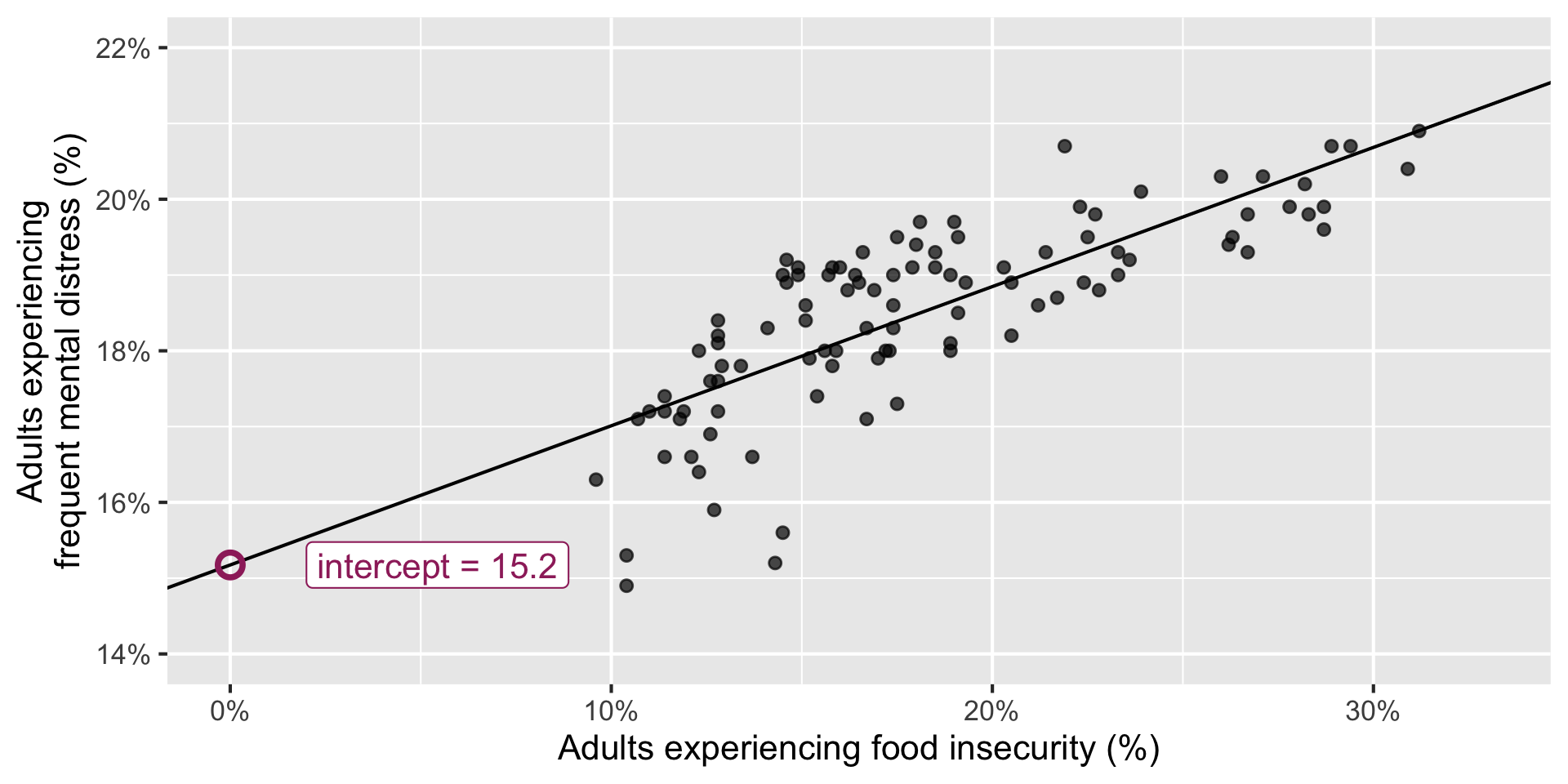
The intercept of the fitted model is 15.2. Which is the best interpretation?

Go to wooclap.com and use the code BSAFXJG.
The intercept is meaningful in context if:
Here, observed food-insecurity prevalence ranges from 9.6% to 31.2%.
Mathematically vs. practical meaningfullness
The intercept is a mathematical part of the line, but it is not meaningful in context.
For a county where 20% of adults experience food insecurity:
\[ \begin{aligned} \widehat{\text{mental distress %}} &= 15.2 + 0.184 \times 20 \\ &= 18.9 \end{aligned} \]
We predict that approximately 18.9% of adults experience frequent mental distress.
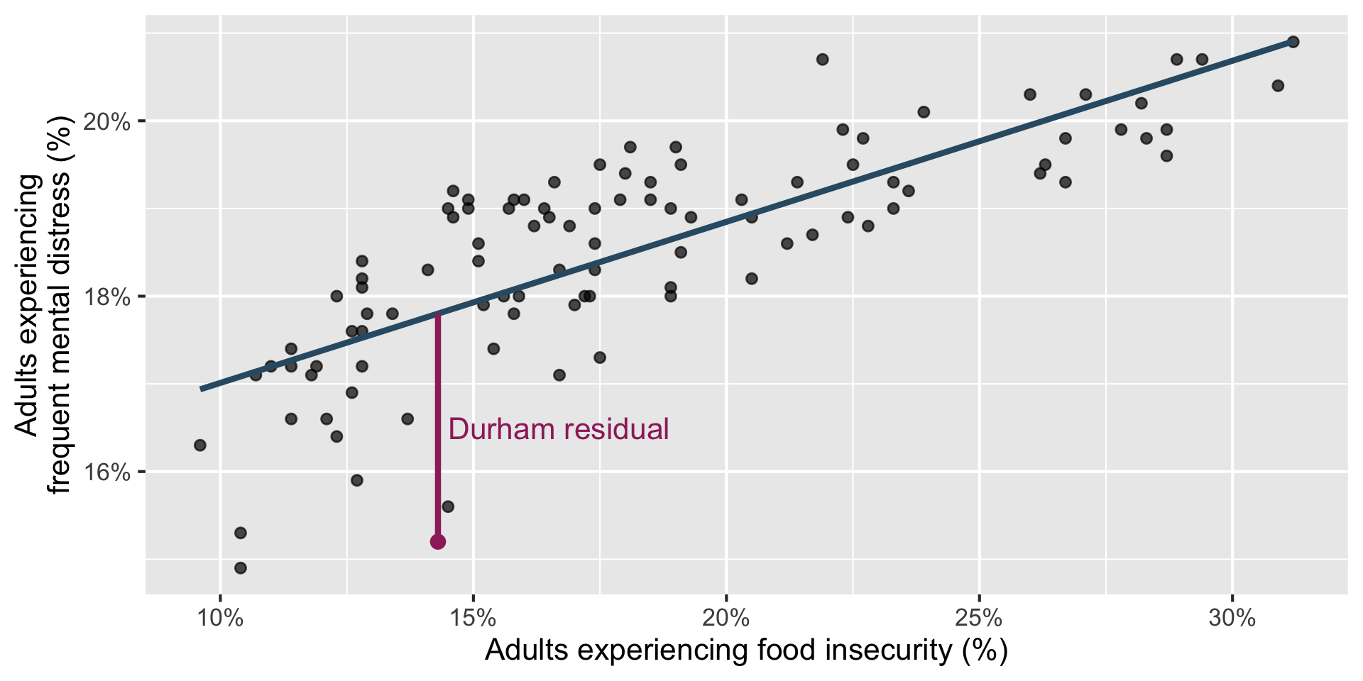
tibble():A residual is the difference between an observed and predicted outcome:
\[ \text{residual} = \text{observed} - \text{predicted} = y - \widehat{y} \]
Use augment() to add predictions and residuals to the original dataset.
# A tibble: 100 Γ 48
.pred .resid county county_fips development_tier region appalachian
<dbl> <dbl> <chr> <dbl> <chr> <chr> <chr>
1 18.3 -0.334 Alamance 37001 Tier 2 Piedmont No
2 18.1 1.02 Alexander 37003 Tier 1 Piedmont Yes
3 18.6 0.728 Alleghany 37005 Tier 2 Mountains Yes
4 20.4 -0.154 Anson 37007 Tier 1 Piedmont No
5 17.9 1.04 Ashe 37009 Tier 2 Mountains Yes
6 17.9 0.452 Avery 37011 Tier 2 Mountains Yes
7 18.7 0.181 Beaufort 37013 Tier 2 Coastal Plain No
8 20.4 -0.846 Bertie 37015 Tier 1 Coastal Plain No
9 19.3 0.193 Bladen 37017 Tier 1 Coastal Plain No
10 17.4 -0.160 Brunswick 37019 Tier 3 Coastal Plain No
# βΉ 90 more rows
# βΉ 41 more variables: food_insecurity <dbl>, mental_distress <dbl>,
# dental_visit <dbl>, fair_or_poor_health <dbl>, all_teeth_lost <dbl>,
# annual_checkup <dbl>, any_disability <dbl>, arthritis <dbl>,
# binge_drinking <dbl>, cancer_non_skin_or_melanoma <dbl>,
# cholesterol_screening <dbl>, cognitive_disability <dbl>,
# colorectal_cancer_screening <dbl>, copd <dbl>, β¦
Which line fits the points bestβand what do we mean by βbestβ?
\[ e_i = y_i - \widehat{y}_i \]
\[ e_1^2 + e_2^2 + \cdots + e_n^2 \]
For a least-squares line with one quantitative predictor and an intercept:
The line passes through the point of means, \((\bar{x}, \bar{y})\): \[b_0 = \bar{y} - b_1\bar{x}\]
The slope and correlation have the same sign: \[b_1 = r\frac{s_y}{s_x}\]
The residuals sum to zero: \[\sum_{i=1}^{n} e_i = 0\]
The residuals and predictor values are uncorrelated.
This model tells us that counties with greater estimated food-insecurity prevalence also tend to have greater estimated mental-distress prevalence.
It does not establish that food insecurity causes mental distress.
Possible explanations include:
Each point is a county, not a person.
An association between two county percentages does not, by itself, establish the same relationship among individuals. This is the ecological fallacy.
Also remember:


Go to your ae project in Positron.
If you havenβt yet done so, make sure all of your changes up to this point are committed and pushed, i.e., thereβs nothing left in your source control pane.
If you havenβt yet done so, pull to get todayβs application exercise file: ae-09-nc-places-model.qmd.
Work through the application exercise in class, and render, commit, and push your edits by the end of class.