Lecture 17
Duke University
STA 199 - Fall 2026
October 26, 2026
Which of the following is true about linear regression models?

Go to wooclap.com and use the code YJMSXJE.
HW 5 due tonight and I have office hours 3:30 - 5 pm
Lab 5 in lab tomorrow:
Extra credit opportunity: Come to office hours AS A FULL TEAM with me or any of the TAs before the final project deadline, share your project progress, and get feedback on next steps. Each team that does this will get 1 extra credit point on the project.
Getting your presentation on your project website:
Create your presentation wherever you want (PowerPoint, Google Slides, Keynote, etc.)
Export as a PDF
Rename the PDF as presentation.pdf (case sensitive)
Place the PDF in your project folder, overwriting the existing, placeholder presentation.pdf file
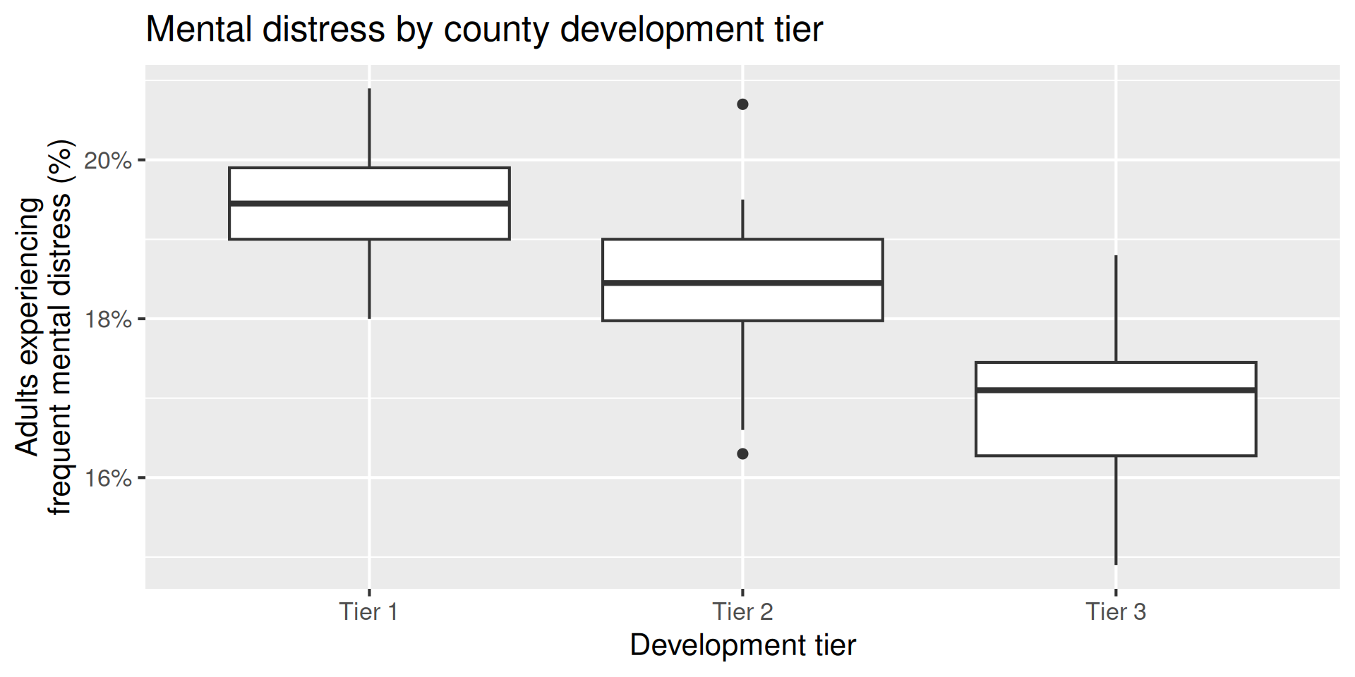
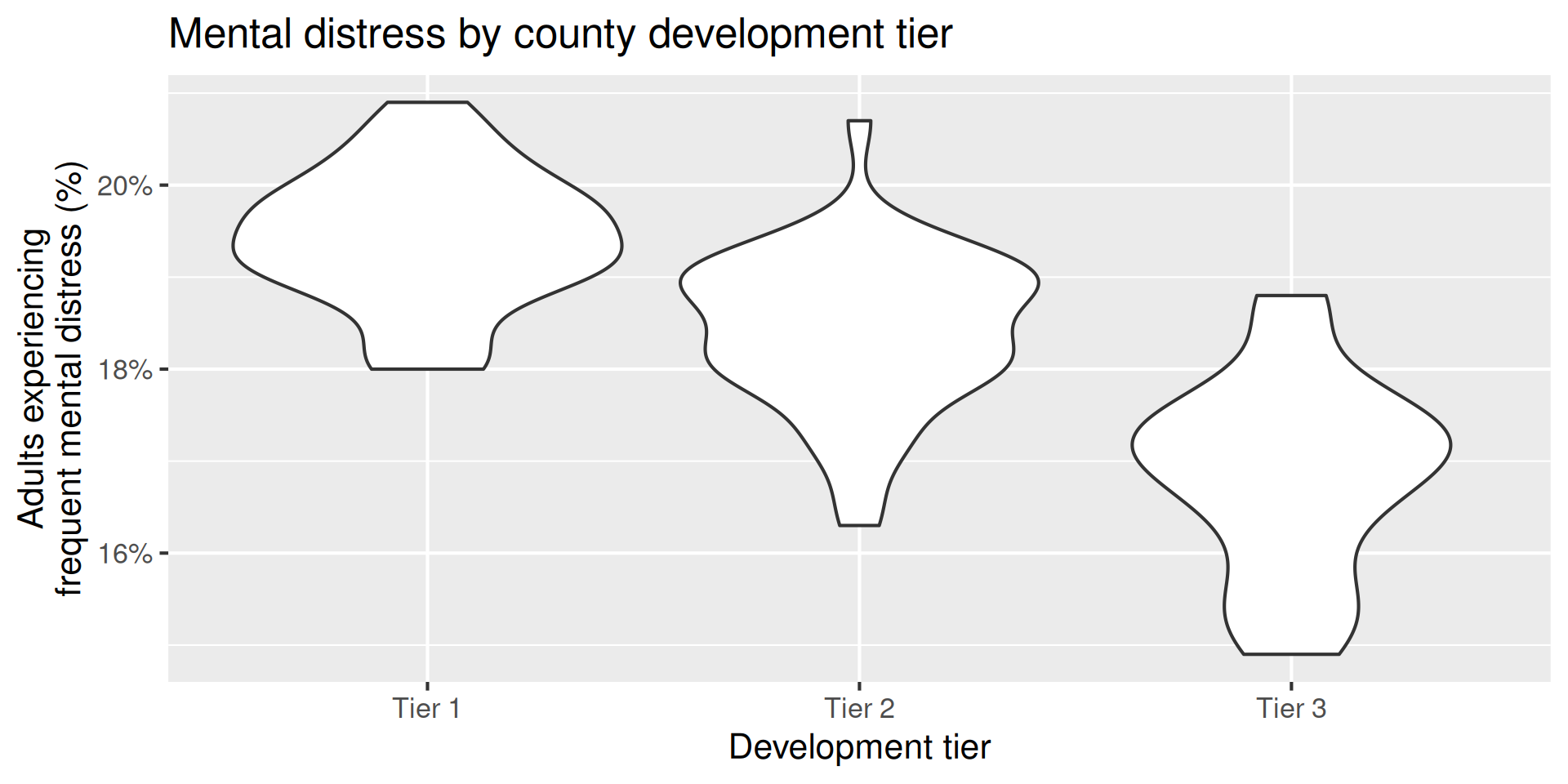
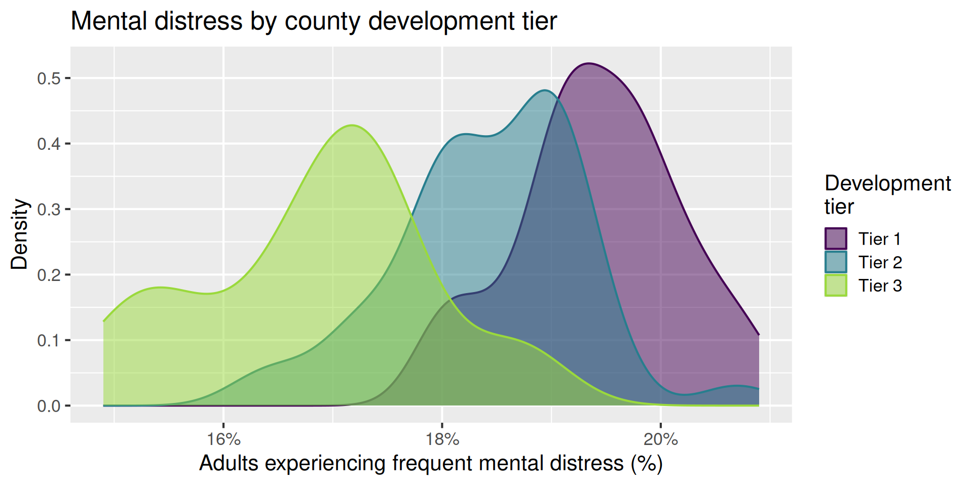
How does estimated frequent mental-distress prevalence vary by county development tier?
outcome: frequent mental-distress prevalence (numerical)
predictor: county development tier (categorical; Tier 1 is most economically distressed and Tier 3 is least economically distressed)
ggplot(
nc_places,
aes(
x = mental_distress,
color = development_tier,
fill = development_tier
)
) +
geom_density(alpha = 0.5) +
scale_x_continuous(labels = label_percent(scale = 1)) +
scale_color_viridis_d(end = 0.85) +
scale_fill_viridis_d(end = 0.85) +
labs(
x = "Adults experiencing frequent mental distress (%)",
y = "Density",
color = "Development\ntier",
fill = "Development\ntier",
title = "Mental distress by county development tier"
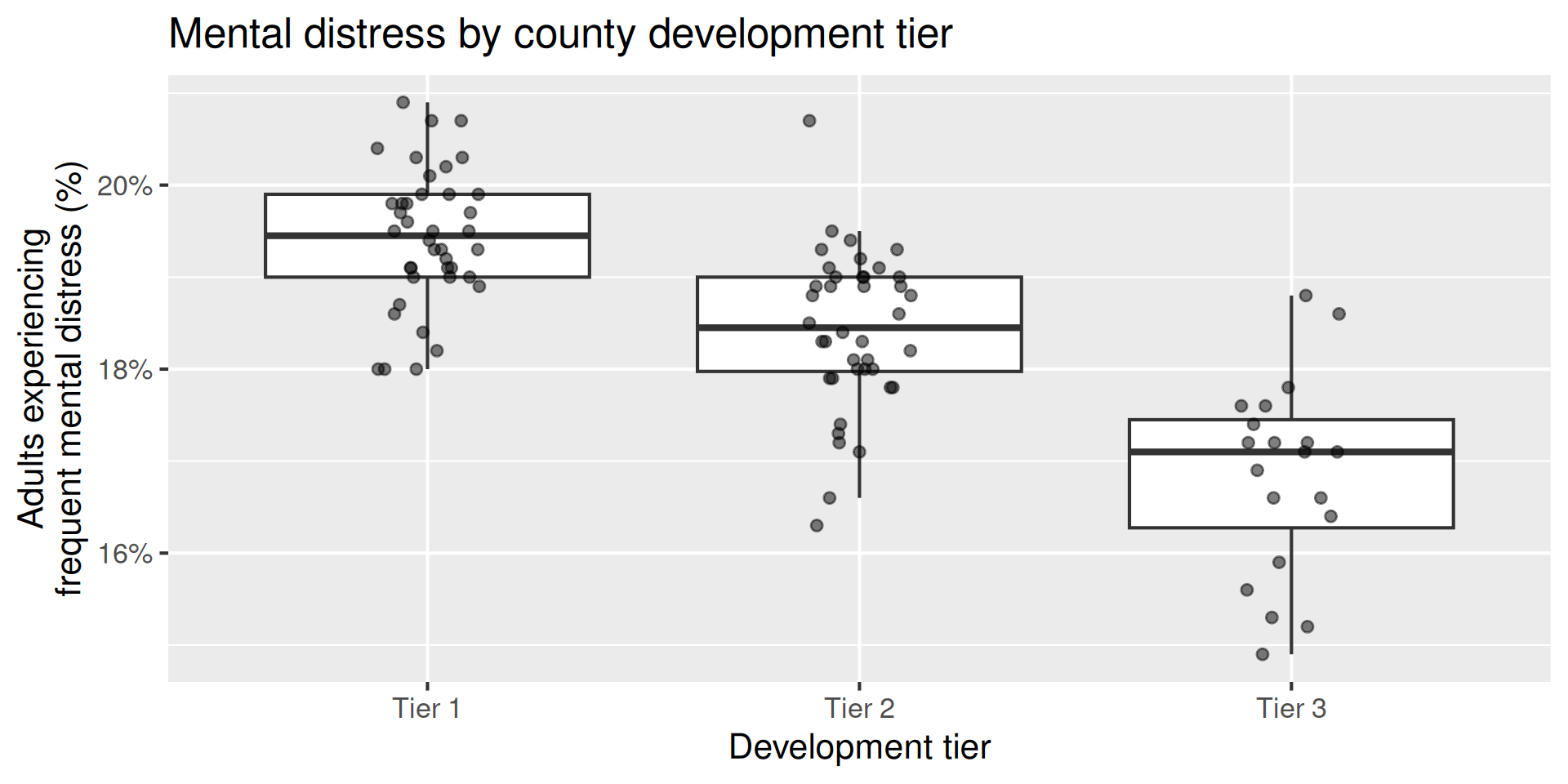
)ggplot(
nc_places,
aes(x = development_tier, y = mental_distress)
) +
geom_boxplot(outlier.shape = NA) +
geom_jitter(width = 0.12, height = 0, size = 2, alpha = 0.5) +
scale_y_continuous(labels = label_percent(scale = 1)) +
labs(
x = "Development tier",
y = "Adults experiencing\nfrequent mental distress (%)",
title = "Mental distress by county development tier"
)Calculate the average mental-distress prevalence for counties in each development tier. How do the averages compare across tiers?
Fit a linear regression model predicting mental-distress prevalence from development tier and display the results.
Why is Tier 1 not in the output?
md_tier_fit <- linear_reg() |>
fit(mental_distress ~ development_tier, data = nc_places)
tidy(md_tier_fit)# A tibble: 3 × 5
term estimate std.error statistic p.value
<chr> <dbl> <dbl> <dbl> <dbl>
1 (Intercept) 19.4 0.136 143. 1.06e-114
2 development_tierTier 2 -1 0.192 -5.22 1.04e- 6
3 development_tierTier 3 -2.57 0.235 -11.0 1.18e- 18
\[ \widehat{\text{mental distress %}} = 19.4 - 1 \times \text{Tier 2} - 2.57 \times \text{Tier 3} \]
\[ \widehat{\text{mental distress %}} = 19.4 \color{#9E2C6A}{- 1 \times \text{Tier 2}} - 2.57 \times \text{Tier 3} \]
Tier 2 counties are predicted to have, on average, a mental-distress prevalence 1 percentage point lower than Tier 1 counties.
\[ \widehat{\text{mental distress %}} = 19.4 - 1 \times \text{Tier 2} \color{#9E2C6A}{- 2.57 \times \text{Tier 3}} \]
Tier 3 counties are predicted to have, on average, a mental-distress prevalence 2.57 percentage points lower than Tier 1 counties.
\[ \widehat{\text{mental distress %}} = \color{#9E2C6A}{19.4} - 1 \times \text{Tier 2} - 2.57 \times \text{Tier 3} \]
The predicted average mental-distress prevalence among Tier 1 counties is 19.4%.
What is the predicted mental-distress prevalence for a Tier 1 county? What are the predicted values for Tier 2 and Tier 3 counties? Where have we seen these values before?
new_counties <- tibble(
county = c("County A", "County B", "County C"),
development_tier = c("Tier 1", "Tier 2", "Tier 3")
)
augment(md_tier_fit, new_data = new_counties)# A tibble: 3 × 3
.pred county development_tier
<dbl> <chr> <chr>
1 19.4 County A Tier 1
2 18.4 County B Tier 2
3 16.8 County C Tier 3
Calculate the predicted mental-distress prevalence for counties in each development tier by hand.
\[ \widehat{\text{mental distress %}} = 19.42 - 1.00 \times \text{Tier 2} - 2.57 \times \text{Tier 3} \]
A categorical predictor is encoded using dummy variables. A predictor with \(k\) levels requires \(k - 1\) dummy variables.
The first level of the categorical variable is the baseline level. In a model with one categorical predictor, the intercept is the predicted value of the outcome for the baseline level (when all dummy variables equal 0).
Each slope coefficient describes the difference between the predicted value of the outcome for that level of the categorical variable compared to the baseline level.
By default, R uses the first level of a categorical variable as the baseline level.
We can change the baseline level by reordering the levels of the categorical variable.

Go to wooclap.com and use the code YJMSXJE.
What is the baseline level of development_tier in the following model?
# A tibble: 3 × 5
term estimate std.error statistic p.value
<chr> <dbl> <dbl> <dbl> <dbl>
1 (Intercept) 18.4 0.136 136. 1.75e-112
2 development_tierTier 1 1.00 0.192 5.22 1.04e- 6
3 development_tierTier 3 -1.57 0.235 -6.70 1.40e- 9

Go to wooclap.com and use the code YJMSXJE.
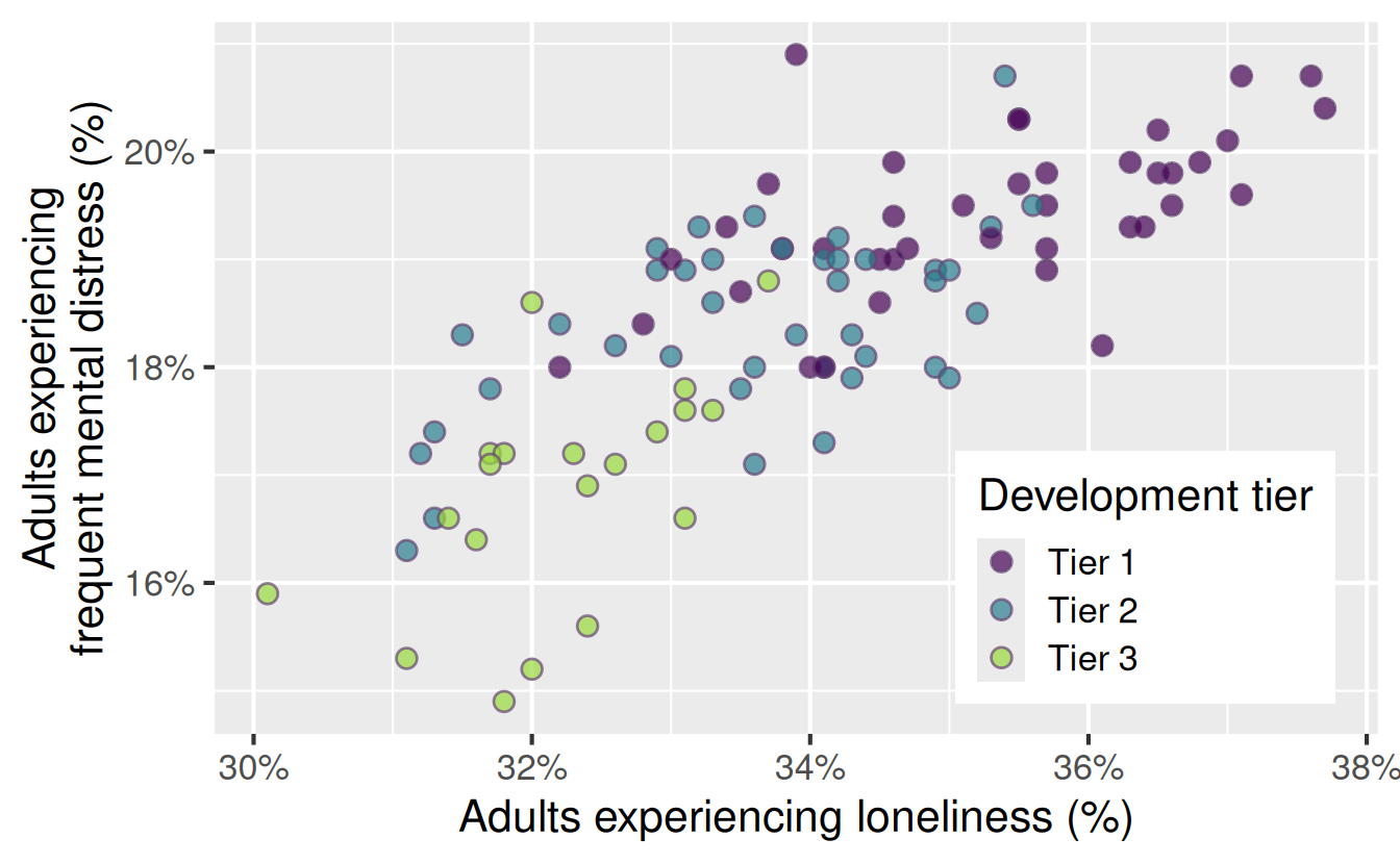
How does estimated frequent mental-distress prevalence vary by county development tier as well as loneliness prevalence?
outcome: frequent mental-distress prevalence (numerical)
predictors:
ggplot(
nc_places,
aes(x = loneliness, y = mental_distress, fill = development_tier)
) +
geom_point(
alpha = 0.7,
size = 3,
shape = "circle filled",
color = "#674574"
) +
scale_x_continuous(labels = label_percent(scale = 1)) +
scale_y_continuous(labels = label_percent(scale = 1)) +
scale_fill_viridis_d(end = 0.85) +
labs(
x = "Adults experiencing loneliness (%)",
y = "Adults experiencing\nfrequent mental distress (%)",
fill = "Development tier",
) +
theme(
legend.position = "inside",
legend.position.inside = c(0.8, 0.22)
)# A tibble: 4 × 5
term estimate std.error statistic p.value
<chr> <dbl> <dbl> <dbl> <dbl>
1 (Intercept) 6.04 2.06 2.93 0.00420
2 development_tierTier 2 -0.381 0.187 -2.04 0.0437
3 development_tierTier 3 -1.41 0.265 -5.33 0.000000651
4 loneliness 0.379 0.0583 6.50 0.00000000352
\[ \begin{aligned} \widehat{\text{mental distress %}} &= 6.04 \\ &- 0.381 \times \text{Tier 2} \\ &- 1.41 \times \text{Tier 3} \\ &+ 0.379 \times \text{loneliness %} \end{aligned} \]
Tier 1: \(\text{Tier 2} = \color{#5C97CB}{\mathbf{0}}\) and \(\text{Tier 3} = \color{#5C97CB}{\mathbf{0}}\)
\[ \begin{aligned} \widehat{\text{mental distress %}} &= 6.04 - 0.381 \times \color{#5C97CB}{\mathbf{0}} - 1.41 \times \color{#5C97CB}{\mathbf{0}} + 0.379 \times \text{loneliness %} \\ &= 6.04 + 0.379 \times \text{loneliness %} \end{aligned} \]
Tier 2: \(\text{Tier 2} = \color{#9E2C6A}{\mathbf{1}}\) and \(\text{Tier 3} = \color{#5C97CB}{\mathbf{0}}\)
\[ \begin{aligned} \widehat{\text{mental distress %}} &= 6.04 - 0.381 \times \color{#9E2C6A}{\mathbf{1}} - 1.41 \times \color{#5C97CB}{\mathbf{0}} + 0.379 \times \text{loneliness %} \\ &= 5.66 + 0.379 \times \text{loneliness %} \end{aligned} \]
Tier 3: \(\text{Tier 2} = \color{#5C97CB}{\mathbf{0}}\) and \(\text{Tier 3} = \color{#9E2C6A}{\mathbf{1}}\)
\[ \begin{aligned} \widehat{\text{mental distress %}} &= 6.04 - 0.381 \times \color{#5C97CB}{\mathbf{0}} - 1.41 \times \color{#9E2C6A}{\mathbf{1}} + 0.379 \times \text{loneliness %} \\ &= 4.63 + 0.379 \times \text{loneliness %} \end{aligned} \]
What do the following look like on a scatterplot?
Tier 1: \(\widehat{\text{mental distress %}} = 6.04 + 0.379 \times \text{loneliness %}\)
Tier 2: \(\widehat{\text{mental distress %}} = 5.66 + 0.379 \times \text{loneliness %}\)
Tier 3: \(\widehat{\text{mental distress %}} = 4.63 + 0.379 \times \text{loneliness %}\)

Go to wooclap.com and use the code YJMSXJE.
md_tier_lone_aug <- augment(
md_tier_lone_fit,
new_data = nc_places
)
ggplot(
md_tier_lone_aug,
aes(x = loneliness, y = mental_distress, fill = development_tier)
) +
geom_line(
aes(y = .pred, color = development_tier),
linewidth = 1
) +
geom_point(
alpha = 0.7,
size = 3,
shape = "circle filled",
color = "#674574"
) +
scale_x_continuous(labels = label_percent(scale = 1)) +
scale_y_continuous(labels = label_percent(scale = 1)) +
scale_color_viridis_d(end = 0.85, guide = "none") +
scale_fill_viridis_d(end = 0.85) +
labs(
x = "Adults experiencing loneliness (%)",
y = "Adults experiencing\nfrequent mental distress (%)",
fill = "Development tier",
title = "Main effects models",
subtitle = "Linear model for each tier: same slope, different intercepts"
) +
theme(
legend.position = "inside",
legend.position.inside = c(0.8, 0.22)
)\[ \begin{aligned} \widehat{\text{mental distress %}} &= 6.04 \\ &- 0.381 \times \text{Tier 2} \\ &- 1.41 \times \text{Tier 3} \\ &+ 0.379 \times \text{loneliness %} \end{aligned} \]
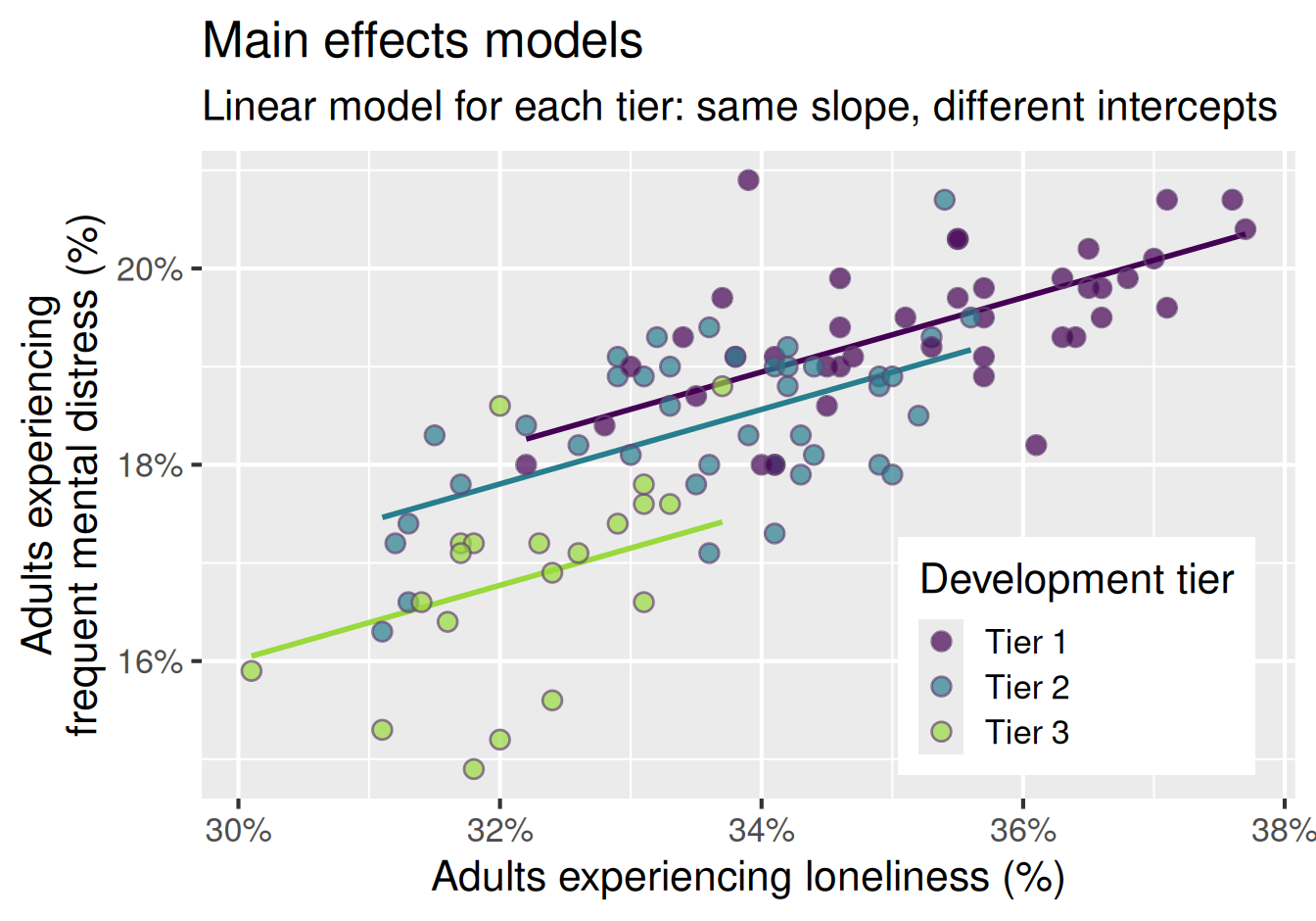
Loneliness: For each additional percentage point in loneliness prevalence, the model predicts mental distress prevalence to be higher, on average, by 0.381 percentage points, all else held constant (i.e., for counties in the same development tier).
\[ \begin{aligned} \widehat{\text{mental distress %}} &= 6.04 \\ &- 0.381 \times \text{Tier 2} \\ &- 1.41 \times \text{Tier 3} \\ &+ 0.379 \times \text{loneliness %} \end{aligned} \]
Tier 2: For Tier 2 counties, the model predicts mental distress prevalence to be lower, on average, by 0.38 percentage points than for Tier 1 counties, all else held constant (i.e., for counties with the same loneliness prevalence).
\[ \begin{aligned} \widehat{\text{mental distress %}} &= 6.04 \\ &- 0.381 \times \text{Tier 2} \\ &- 1.41 \times \text{Tier 3} \\ &+ 0.379 \times \text{loneliness %} \end{aligned} \]
Tier 3: For Tier 3 counties, the model predicts mental distress prevalence to be lower, on average, by 1.41 percentage points than for Tier 1 counties, all else held constant (i.e., for counties with the same loneliness prevalence).
\[ \begin{aligned} \widehat{\text{mental distress %}} &= 6.04 \\ &- 0.381 \times \text{Tier 2} \\ &- 1.41 \times \text{Tier 3} \\ &+ 0.379 \times \text{loneliness %} \end{aligned} \]
Intercept: For Tier 1 counties with 0% loneliness prevalence, the model predicts mental distress prevalence to be 6.04%. However, 0% loneliness is outside the range of the observed data, so the intercept is not meaningful in context.
How much of the variability in mental-distress prevalence is explained by…
tier alone:
The model with tier alone as predictor explains approximately 55.4% of the variability in mental-distress prevalence among North Carolina counties.
What does this say about which model is better for predicting mental distress prevalence?
tier alone:
What does this say about which model is better for predicting mental distress prevalence?
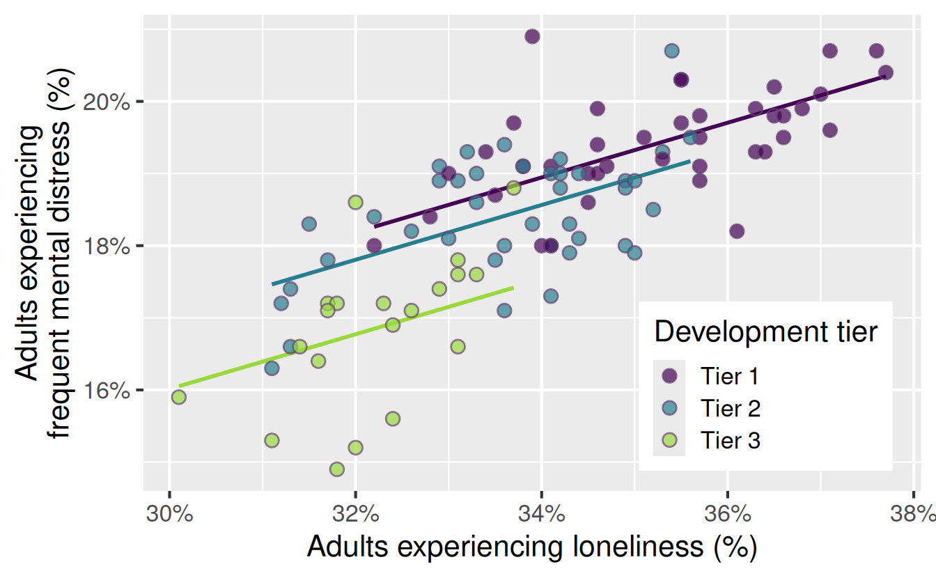
Current model: Mental distress prevalence is higher by the same amount for each additional percentage point in loneliness prevalence, regardless of development tier.
Could there be a different reality?
md_tier_lone_aug <- augment(
md_tier_lone_fit,
new_data = nc_places
)
ggplot(
md_tier_lone_aug,
aes(x = loneliness, y = mental_distress, fill = development_tier)
) +
geom_line(
aes(y = .pred, color = development_tier),
linewidth = 1
) +
geom_point(
alpha = 0.7,
size = 3,
shape = "circle filled",
color = "#674574"
) +
scale_x_continuous(labels = label_percent(scale = 1)) +
scale_y_continuous(labels = label_percent(scale = 1)) +
scale_color_viridis_d(end = 0.85, guide = "none") +
scale_fill_viridis_d(end = 0.85) +
labs(
x = "Adults experiencing loneliness (%)",
y = "Adults experiencing\nfrequent mental distress (%)",
fill = "Development tier",
) +
theme(
legend.position = "inside",
legend.position.inside = c(0.8, 0.22)
)

Go to your ae project in Positron.
If you haven’t yet done so, make sure all of your changes up to this point are committed and pushed, i.e., there’s nothing left in your source control pane.
If you haven’t yet done so, pull to get today’s application exercise file: ae-10-nc-places-multi-model.qmd.
Work through the application exercise in class, and render, commit, and push your edits by the end of class.