AE 10: Mental distress with multiple predictors

Getting started

Packages

We will use the tidyverse package for data visualization and wrangling, the tidymodels package for modeling, and the scales package for formatting percentages.

library(tidyverse)
library(tidymodels)
library(scales)

Data

The data can be found in the data folder; the file is called nc-places.csv.

nc_places <- read_csv("data/nc-places.csv")

The variables used in this exercise are:

Variable name	Description
`county`	North Carolina county name
`development_tier`	County development tier; Tier 1 is the most economically distressed and Tier 3 is the least economically distressed
`loneliness`	Percentage of adults reporting that they always, usually, or sometimes feel lonely
`mental_distress`	Percentage of adults experiencing frequent mental distress

The percentage variables are age-adjusted, model-based estimates.

The main-effects model

So far, we fit the following main effects model:

md_tier_lone_main_fit <- linear_reg() |>
  fit(
    mental_distress ~ development_tier + loneliness,
    data = nc_places
  )

tidy(md_tier_lone_main_fit)

# A tibble: 4 × 5
  term                   estimate std.error statistic       p.value
  <chr>                     <dbl>     <dbl>     <dbl>         <dbl>
1 (Intercept)               6.04     2.06        2.93 0.00420      
2 development_tierTier 2   -0.381    0.187      -2.04 0.0437       
3 development_tierTier 3   -1.41     0.265      -5.33 0.000000651  
4 loneliness                0.379    0.0583      6.50 0.00000000352

In this model, what assumption do we make about the relationship between loneliness and mental distress across the three development tiers?

The main-effects model assumes that the relationship has the same slope in all three development tiers. The fitted lines are parallel: tier may change the predicted level of mental distress, but it does not change the predicted rate of increase in mental distress as loneliness increases.

Could the slopes differ?

The following plot also fits a separate regression line for each development tier.

Remembering what each tier represents can be helpful:

Tier 1: 40 most economically distressed counties
Tier 2: next 40 counties
Tier 3: 20 least economically distressed counties

ggplot(
  nc_places,
  aes(x = loneliness, y = mental_distress, color = development_tier)
) +
  geom_point(alpha = 0.7) +
  geom_smooth(method = "lm", se = FALSE) +
  scale_x_continuous(labels = label_percent(scale = 1)) +
  scale_y_continuous(labels = label_percent(scale = 1)) +
  scale_color_viridis_d(end = 0.85) +
  labs(
    x = "Adults experiencing loneliness (%)",
    y = "Adults experiencing frequent mental distress (%)",
    color = "Development tier"
  ) +
  theme(legend.position = "bottom")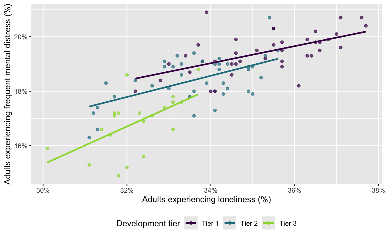

How do these lines differ from the parallel fitted lines produced by the main effects model?

These lines are not constrained to be parallel. Each development tier has its own intercept and its own loneliness slope. The Tier 3 line is noticeably steeper than the Tier 1 and Tier 2 lines.

Fitting an interaction model

An interaction effects model allows the slope for loneliness to differ across development tiers. In a model formula, development_tier * loneliness includes:

the main effect of development_tier,
the main effect of loneliness, and
their interaction.
Fit the interaction model and examine its coefficients. Name the model md_tier_lone_int.

md_tier_lone_int <- linear_reg() |>
  fit(
    mental_distress ~ development_tier * loneliness,
    data = nc_places
  )

tidy(md_tier_lone_int)

# A tibble: 6 × 5
  term                              estimate std.error statistic  p.value
  <chr>                                <dbl>     <dbl>     <dbl>    <dbl>
1 (Intercept)                         8.39      2.89       2.91  0.00457 
2 development_tierTier 2             -3.05      4.21      -0.725 0.471   
3 development_tierTier 3            -13.9       6.75      -2.06  0.0424  
4 loneliness                          0.313     0.0818     3.83  0.000233
5 development_tierTier 2:loneliness   0.0761    0.122      0.622 0.535   
6 development_tierTier 3:loneliness   0.381     0.206      1.85  0.0678

Which development tier is the baseline level?

Tier 1 is the baseline level. It does not appear as a separate indicator term in the model output.

Comparing the two models visually

Set the following code cell’s eval option to true to render the visualizations of main and interaction effect models. Describe what the code is doing.

md_tier_lone_main_aug <- augment(
  md_tier_lone_main_fit,
  new_data = nc_places
)

ggplot(
  md_tier_lone_main_aug,
  aes(x = loneliness, color = development_tier)
) +
  geom_point(aes(y = mental_distress), alpha = 0.5) +
  geom_line(aes(y = .pred), linewidth = 1) +
  scale_color_viridis_d(end = 0.85) +
  labs(
    x = "Loneliness (%)",
    y = "Mental distress (%)",
    color = "Development tier",
    title = "Main-effects model"
  ) +
  theme(legend.position = "bottom")
md_tier_lone_int_aug <- augment(
  md_tier_lone_int,
  new_data = nc_places
)

ggplot(
  md_tier_lone_int_aug,
  aes(x = loneliness, color = development_tier)
) +
  geom_point(aes(y = mental_distress), alpha = 0.5) +
  geom_line(aes(y = .pred), linewidth = 1) +
  scale_color_viridis_d(end = 0.85) +
  labs(
    x = "Loneliness (%)",
    y = "Mental distress (%)",
    color = "Development tier",
    title = "Interaction model"
  ) +
  theme(legend.position = "bottom")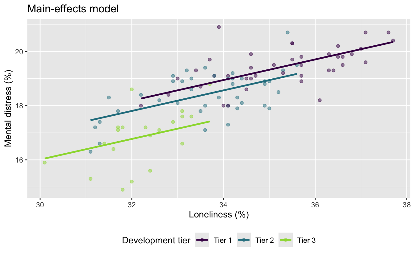

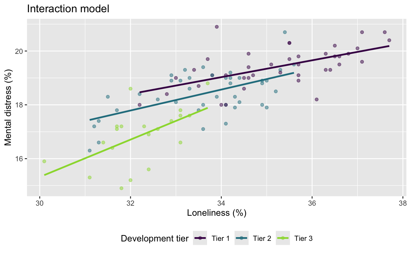
The code first uses augment() to add each model’s predictions to the county data. It then plots the observed county values and connects the fitted values within each development tier. The main-effects plot shows predictions from the model with a common loneliness slope, while the interaction plot shows predictions from the model with a separate slope for each tier.

Describe the key difference between the fitted lines in the two plots.

The main-effects model produces three parallel lines with the same loneliness slope. The interaction model produces three lines with different slopes; the Tier 3 line is the steepest.

Which model makes the stronger assumption about the relationship between loneliness and mental distress? Explain.

The main-effects model makes the stronger assumption because it requires the loneliness slope to be the same for all three tiers. The interaction model is more flexible because it allows the slope to vary by tier.

Interpreting the interaction model

Write the fitted interaction model using mathematical notation. Your model should contain six coefficient estimates.

\[ \begin{aligned} \widehat{\text{mental distress %}} &= 8.39 - 3.05 \times \text{Tier 2} - 13.90 \times \text{Tier 3} \\ &\quad + 0.313 \times \text{loneliness %} \\ &\quad + 0.076 \times (\text{Tier 2} \times \text{loneliness %}) \\ &\quad + 0.381 \times (\text{Tier 3} \times \text{loneliness %}) \end{aligned} \]

Write the model for Tier 1 counties using mathematical notation. Then, interpret the slope for loneliness in context.

For Tier 1 counties, both tier indicators equal 0:

\[ \widehat{\text{mental distress %}} = 8.39 + 0.313 \times \text{loneliness %} \]

Among Tier 1 counties, each additional percentage point in loneliness prevalence is associated with a predicted 0.313 percentage-point increase in mental-distress prevalence, on average.

Write the model for Tier 2 counties using mathematical notation. Then, interpret the slope for loneliness in context.

For Tier 2 counties, the intercept is (8.39 - 3.05 = 5.34), and the loneliness slope is (0.313 + 0.076 = 0.389):

\[ \widehat{\text{mental distress %}} = 5.34 + 0.389 \times \text{loneliness %} \]

Among Tier 2 counties, each additional percentage point in loneliness prevalence is associated with a predicted 0.389 percentage-point increase in mental-distress prevalence, on average.

Write the model for Tier 3 counties using mathematical notation. Then, interpret the slope for loneliness in context.

For Tier 3 counties, the intercept is (8.39 - 13.90 = -5.51), and the loneliness slope is (0.313 + 0.381 = 0.694):

\[ \widehat{\text{mental distress %}} = -5.51 + 0.694 \times \text{loneliness %} \]

Among Tier 3 counties, each additional percentage point in loneliness prevalence is associated with a predicted 0.694 percentage-point increase in mental-distress prevalence, on average.

In the interaction model, what does the intercept represent? Is its interpretation meaningful for these data?

The intercept predicts a mental-distress prevalence of 8.39% for a Tier 1 county with 0% loneliness. This is not meaningful in context because observed loneliness prevalences range from approximately 30.1% to 37.7%; 0% is far outside the observed data.

Comparing model fit

Calculate the \(R^2\) and adjusted \(R^2\) for each model.

bind_rows(
  glance(md_tier_lone_main_fit) |>
    mutate(model = "Main effects"),
  glance(md_tier_lone_int) |>
    mutate(model = "Interaction effects")
) |>
  select(model, r.squared, adj.r.squared)

# A tibble: 2 × 3
  model               r.squared adj.r.squared
  <chr>                   <dbl>         <dbl>
1 Main effects            0.691         0.681
2 Interaction effects     0.702         0.686

Which model has the higher \(R^2\)? Why does adding interaction terms necessarily result in an \(R^2\) that is at least as high?

The interaction model has the higher (R^2): approximately 0.702, compared with 0.691 for the main-effects model. The interaction model contains all the terms in the main-effects model plus two additional terms. Those terms give it more flexibility to fit the observed data; if they are not helpful, their coefficients can effectively be 0, so (R^2) cannot decrease.

Which model has the higher adjusted \(R^2\)? Why is adjusted \(R^2\) more useful than \(R^2\) for this comparison?

The interaction model also has the higher adjusted (R^2), approximately 0.686 versus 0.681. Adjusted (R^2) penalizes a model for adding predictor coefficients, so it helps determine whether the improvement in fit is sufficient to offset the additional complexity.

How large is the difference in fit between the two models? Do you consider this difference practically meaningful?

The differences are small: (R^2) increases by about 0.011, and adjusted (R^2) increases by about 0.005. The interaction model explains only about one additional percentage point of variability, so the practical improvement is modest.

Considering both model fit and simplicity, which model would you choose for predicting mental-distress prevalence? Justify your choice.

A reasonable choice is the main-effects model. Its fit is nearly as good, it uses two fewer coefficients, and its parallel lines are easier to communicate. Choosing the interaction model is also defensible if tier-specific rates of change are substantively important, but the improvement in fit is small.