AE 11: Predicting Dem flips
Suggested answers
These are suggested answers. This document should be used as reference only, it’s not designed to be an exhaustive key.
In this application exercise, we will
- Fit a logistic regression model for a binary response variable in R
- Use a logistic regression model to predict probabilities and classify new observations
- Compare logistic regression models using AIC
We will predict whether a U.S. House seat flipped to Democrat in the 2026 midterm elections, using data from Decision Desk HQ as of 2026-11-04 at 11:14 am. At that time, some races had been called and others had not. We’ll learn from the called races and make predictions for the uncalled ones.
midterm_26 <- read_csv("data/midterm-26.csv")Rows: 435 Columns: 19
── Column specification ────────────────────────────────────────────────────────
Delimiter: ","
chr (15): district, state_abb, state, house_rep_20, house_party_20, house_re...
dbl (4): harris_24, trump_24, margin_26, flip_dem_24_26
ℹ Use `spec()` to retrieve the full column specification for this data.
ℹ Specify the column types or set `show_col_types = FALSE` to quiet this message.glimpse(midterm_26)Rows: 435
Columns: 19
$ district <chr> "AK-00", "AL-01", "AL-02", "AL-03", "AL-04", "AL-05", "…
$ state_abb <chr> "AK", "AL", "AL", "AL", "AL", "AL", "AL", "AL", "AR", "…
$ state <chr> "Alaska", "Alabama", "Alabama", "Alabama", "Alabama", "…
$ house_rep_20 <chr> "Don Young", "Jerry Carl", "Barry Moore", "Mike Rogers"…
$ house_party_20 <chr> "Republican", "Republican", "Republican", "Republican",…
$ house_rep_22 <chr> "Mary Sattler Peltola", "Jerry L Carl", "Barry Moore", …
$ house_party_22 <chr> "Democrat", "Republican", "Republican", "Republican", "…
$ house_rep_24 <chr> "Nick Begich", "Barry Moore", "Shomari Figures", "Mike …
$ house_party_24 <chr> "Republican", "Republican", "Democrat", "Republican", "…
$ harris_24 <dbl> 41.41, 21.89, 53.52, 26.18, 15.96, 34.20, 29.68, 61.45,…
$ trump_24 <dbl> 54.54, 76.94, 45.31, 72.71, 83.02, 64.02, 68.47, 37.50,…
$ gerry_22 <chr> NA, "F", "F", "F", "F", "F", "F", "F", "C", "C", "C", "…
$ gerry_24 <chr> NA, "B", "B", "B", "B", "B", "B", "B", "C", "C", "C", "…
$ gerry_26 <chr> NA, "B", "B", "B", "B", "B", "B", "B", "C", "C", "C", "…
$ rating_26 <chr> "Lean R", "Safe R", "Lean R", "Safe R", "Safe R", "Safe…
$ leader_26 <chr> "Republican", "Republican", "Democrat", "Republican", "…
$ margin_26 <dbl> 9.00, 18.00, 8.00, 28.00, 50.00, 7.00, 15.00, 39.00, 35…
$ called_26 <chr> "uncalled", "called", "called", "called", "called", "ca…
$ flip_dem_24_26 <dbl> NA, 0, 0, 0, 0, 0, 0, 0, 0, 0, 0, 0, NA, NA, 0, 0, NA, …The variables we’ll use in this analysis are
-
district: Congressional district -
called_26: Whether the 2026 race had been called (called) or not (uncalled) -
flip_dem_24_26: 1 if the seat was held by a Republican after 2024 and a Democrat leads in 2026, 0 otherwise (NAfor uncalled races) -
trump_24: Trump’s 2024 vote share (%) in the district -
gerry_26: Grade (A-F) of the state’s 2026 congressional map from the Redistricting Report Card, where A is the fairest and F is the most gerrymandered
Goal: Use Trump’s 2024 vote share and the state’s gerrymandering grade to predict whether a seat flips to Democrat.
Data prep
Make flip_dem_24_26 a factor (so we can use it as the outcome of a logistic regression model), and split the data into called and uncalled races.
How many called and uncalled races are there?
midterm_26 |>
  count(called_26)
# A tibble: 2 × 2
called_26 n
<chr> <int>
1 called 391
2 uncalled 44391 called and 44 uncalled.
Exercises
Exercise 1
- Among the called races, how many seats flipped to Democrat?
midterm_called |>
  count(flip_dem_24_26)
# A tibble: 2 × 2
flip_dem_24_26 n
<fct> <int>
1 0 353
2 1 3838 of the 391 called seats flipped to Democrat.
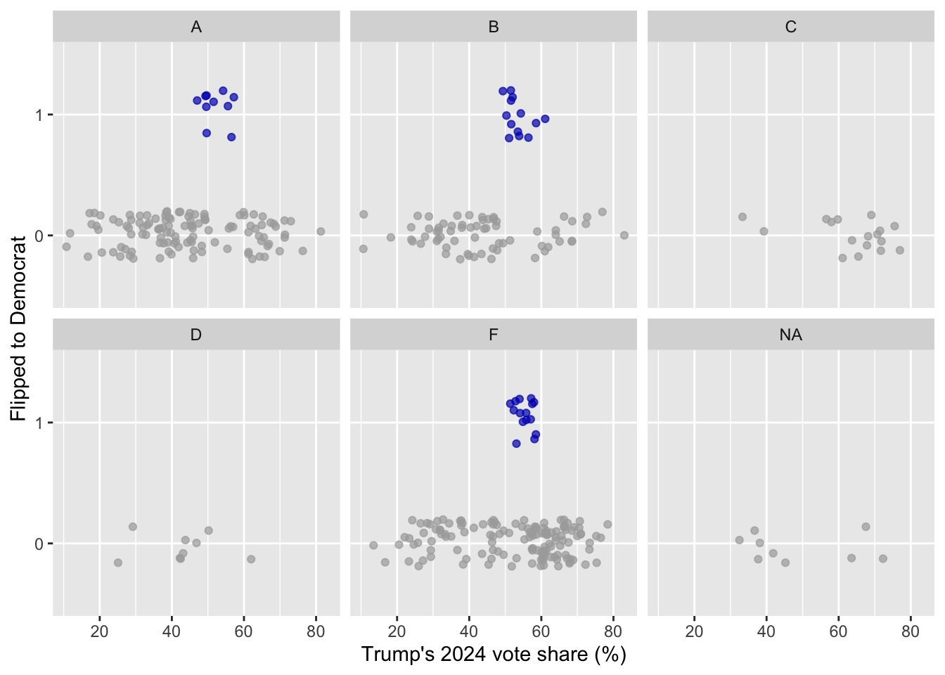
- Calculate the proportion of called seats that flipped to Democrat for each gerrymandering grade. What do you notice?
# A tibble: 9 × 4
# Groups:   gerry_26 [6]
  gerry_26 flip_dem_24_26     n      p
  <chr>    <fct>          <int>  <dbl>
1 A        0                115 0.92
2 A        1                 10 0.08
3 B        0                 66 0.835
4 B        1                 13 0.165
5 C        0                 17 1
6 D        0                  9 1
7 F        0                137 0.901
8 F        1                 15 0.0987
9 <NA>     0                  9 1
None of the seats in states with C or D grades flipped. The proportion of flips is highest in states with a B grade.
- Visualize the relationship between
trump_24,gerry_26, andflip_dem_24_26for the called races.
ggplot(
  midterm_called,
  aes(x = trump_24, y = flip_dem_24_26, color = flip_dem_24_26)
) +
  geom_jitter(height = 0.2, alpha = 0.7, show.legend = FALSE) +
  facet_wrap(~gerry_26) +
  scale_color_manual(values = c("0" = "darkgray", "1" = "#0015BC")) +
  labs(
    x = "Trump's 2024 vote share (%)",
    y = "Flipped to Democrat"
  )
Exercise 2
- Fit a logistic regression model predicting
flip_dem_24_26fromtrump_24andgerry_26using the called races.
flip_gerry_fit <- logistic_reg() |>
  fit(flip_dem_24_26 ~ trump_24 + gerry_26, data = midterm_called)

tidy(flip_gerry_fit)
# A tibble: 6 × 5
term estimate std.error statistic p.value
<chr> <dbl> <dbl> <dbl> <dbl>
1 (Intercept) -3.93 0.716 -5.48 0.0000000419
2 trump_24 0.0310 0.0125 2.49 0.0129
3 gerry_26B 0.823 0.453 1.82 0.0694
4 gerry_26C -15.6 951. -0.0164 0.987
5 gerry_26D -15.0 1308. -0.0115 0.991
6 gerry_26F 0.00685 0.438 0.0156 0.988 - Write out the fitted model for the log-odds.
\[ \log\left(\frac{\hat{p}}{1-\hat{p}}\right) = -3.93 + 0.0310 \times trump\_24 + 0.823 \times gerry\_26B - 15.6 \times gerry\_26C - 15.0 \times gerry\_26D + 0.00685 \times gerry\_26F \]
- Interpret the coefficient for
gerry_26Bin terms of odds.
Holding Trump’s 2024 vote share constant, seats in states with a B-graded map are predicted to have odds of flipping to Democrat that are higher by a factor of \(e^{0.823} \approx 2.28\) compared to seats in states with an A-graded map, on average.
- The coefficients for
gerry_26Candgerry_26Dare very large and negative, with huge standard errors. Why? Hint: Look back at your answer to Exercise 1b.
None of the called seats in states with C or D grades flipped, so the model pushes the predicted probability of a flip for these seats as close to 0 as it can.
Exercise 3
NY-17 is one of the uncalled races.
- What are Trump’s 2024 vote share and the gerrymandering grade for NY-17?
# A tibble: 1 × 3
  district trump_24 gerry_26
  <chr>       <dbl> <chr>
1 NY-17 49.4 A - What is the predicted probability that NY-17 flips to Democrat? Answer the question using the
predict()function with the appropriatetypeargument.
predict(flip_gerry_fit, new_data = ny_17, type = "prob")# A tibble: 1 × 2
.pred_0 .pred_1
<dbl> <dbl>
1 0.917 0.0834About 0.08.
- A probability is nice, but we want an actual decision. Classify NY-17. What threshold does
predict()use by default?
predict(flip_gerry_fit, new_data = ny_17, type = "class")# A tibble: 1 × 1
.pred_class
<fct>
1 0 The model predicts NY-17 doesn’t flip (0). The default threshold is 0.5.
- Now try AK-00, another uncalled race. What happens, and why?
# A tibble: 1 × 3
  district trump_24 gerry_26
  <chr>       <dbl> <chr>
1 AK-00 54.5 <NA> predict(flip_gerry_fit, new_data = ak_00, type = "prob")# A tibble: 1 × 2
.pred_0 .pred_1
<dbl> <dbl>
1 NA NAThe prediction is NA because Alaska has a single at-large district, so it doesn’t have a gerrymandering grade. The model can’t make a prediction without a value for every predictor.
Exercise 4
- Predict the probability of flipping to Democrat and classify all uncalled races. How many are predicted to flip to Democrat?
flip_uncalled_aug <- augment(flip_gerry_fit, new_data = midterm_uncalled)

flip_uncalled_aug |>
  count(.pred_class)
# A tibble: 2 × 2
.pred_class n
<fct> <int>
1 0 43
2 <NA> 1None! All predicted probabilities are below 0.5.
- Which uncalled races have the highest predicted probability of flipping to Democrat?
# A tibble: 44 × 5
   district trump_24 gerry_26 house_party_24 .pred_1
   <chr>       <dbl> <chr>    <chr>            <dbl>
 1 CA-05        57.6 B        Republican       0.211
 2 CA-23        57.1 B        Republican       0.209
 3 ME-02        53.8 B        Democrat         0.192
 4 CA-40        49.5 B        Republican       0.172
 5 TN-04        71.2 F        Republican       0.153
 6 FL-26        67.0 F        Republican       0.137
 7 TX-27        64.4 F        Republican       0.127
 8 TX-02        61.3 F        Republican       0.117
 9 NC-03        60.3 F        Republican       0.114
10 NY-21        60.1 A        Republican       0.113
# ℹ 34 more rows
CA-05, CA-23, and ME-02 have the highest predicted probabilities, around 0.2. Note that ME-02 was held by a Democrat after 2024, so it can’t flip to Democrat. Our model doesn’t know that!
- The overall proportion of called seats that flipped is about 0.1. Classify the uncalled races again, this time using 0.1 as the threshold. How many are predicted to flip now?
# A tibble: 3 × 2
  .pred_class_10     n
           <dbl> <int>
1              0    16
2              1    27
3             NA     1
27 uncalled races are predicted to flip to Democrat with a threshold of 0.1.
Exercise 5
In the slides, we fit a model predicting flip_dem_24_26 from trump_24 only. Is the model with gerry_26 better?
- Fit the model from the slides, then compare the AIC values of the two models using
glance().
flip_trump_fit <- logistic_reg() |>
  fit(flip_dem_24_26 ~ trump_24, data = midterm_called)

glance(flip_trump_fit)
# A tibble: 1 × 8
null.deviance df.null logLik AIC BIC deviance df.residual nobs
<dbl> <int> <dbl> <dbl> <dbl> <dbl> <int> <int>
1 249. 390 -122. 249. 257. 245. 389 391glance(flip_gerry_fit)# A tibble: 1 × 8
null.deviance df.null logLik AIC BIC deviance df.residual nobs
<dbl> <int> <dbl> <dbl> <dbl> <dbl> <int> <int>
1 247. 381 -116. 244. 267. 232. 376 382- Take a look at the
nobscolumn in the output. Why can’t we compare these AIC values directly?
The trump_24 model was fit to all 391 called seats, but the gerry_26 model was fit to only 382, because the 9 called seats with no gerrymandering grade were dropped. AIC can only be compared between models fit to the same data.
- Refit both models on the called seats that have a gerrymandering grade, and compare the AIC values. Which model is better?
midterm_called_graded <- midterm_called |>
  filter(!is.na(gerry_26))

flip_trump_fit_graded <- logistic_reg() |>
  fit(flip_dem_24_26 ~ trump_24, data = midterm_called_graded)

flip_gerry_fit_graded <- logistic_reg() |>
  fit(flip_dem_24_26 ~ trump_24 + gerry_26, data = midterm_called_graded)

glance(flip_trump_fit_graded)$AIC
[1] 246.9217glance(flip_gerry_fit_graded)$AIC[1] 243.6752The model with gerry_26 has a lower AIC (244.0 vs. 246.9), so it is the better model, though not by much.