Hello, World!
Lecture 1
Hello world!
Meet the prof
Dr. Mine Çetinkaya-Rundel
Professor of the Practice
Director of First-Year Experience in Trinity College of Arts & Sciences
Associate Director of Undergraduate Studies, Statistical Science
Office: Old Chem 211C
Office hours:
- 3:30-5 pm on Wednesdays at my office
- Always available after class
- Also available by appointment
Meet the course team
- Mary Knox (Course coordinator)
- Josh Lim (PhD) (Head TA)
- Helen Chen (PhD)
- Cael Elmore (PhD)
- Robbie Hao (MS)
- Carl Emerson (MS)
- Juan Pablo Lopez Escamilla (MS)
- Kenna Roberts (MS)
- Yasmine Abdel-Rahman (UG)
- Tally Coulter (UG)
- Oliver Gao (UG)
- Hellen Han (UG)
- Hyunjin Lee (UG)
- Anric Ngan (UG)
- Chelsea Nguyen (UG)
- Max Niu (UG)
- Sophie Schwartz (UG)
- Allison Yang (UG)
Meet each other!
Please share with at least two classmates…
- Your name
- Your year
- Where you’re from
- What you did this past summer
- What you hope to get out of this course
Meet data science
Data science is an exciting discipline that allows you to turn raw data into understanding, insight, and knowledge.
We’re going to learn to do this in a modern and
tidyway – more on that later!This is a course on introduction to data science, with an emphasis on statistical thinking.
Hello, country music! 🎸
Let’s do some data science!
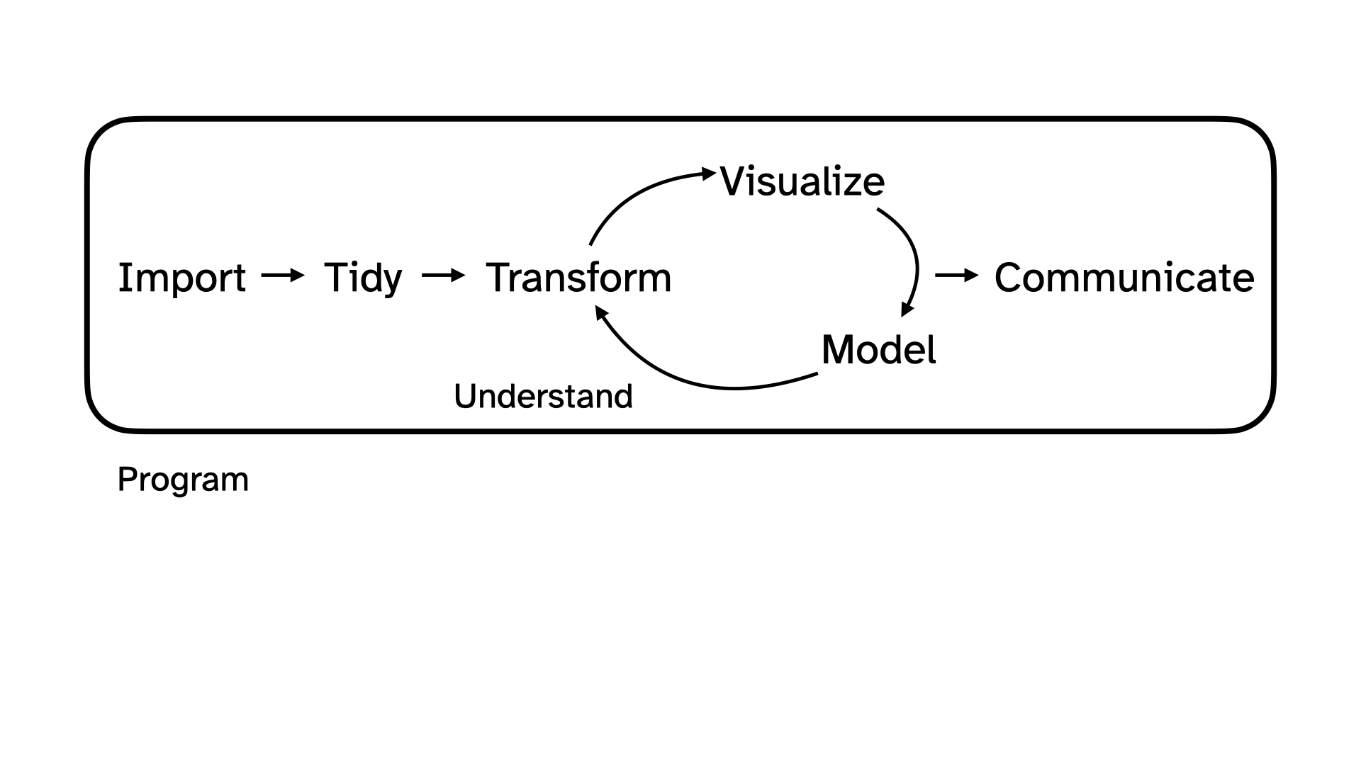
Today we’re going to explore some data together, following the data science cycle.
Our question: Are the stereotypes about country music actually true?
Participate 💻📱
Scan the QR code or go to wooclap.com. Log in with your Duke NetID and enter the code OQPLQEK.
Are the stereotypes about country music actually true?
“Is it REALLY all about beer and trucks and girls and blue jeans? Are all the lyrics REALLY the same?”
— Grady Smith, country music critic
Data
Grady Smith kept a spreadsheet of every country song that reached the Top 30 of Billboard’s Country Airplay chart.
Someone tidied it up and put it in a CSV (comma-separated values) file and released it as part of the TidyTuesday project.
Import
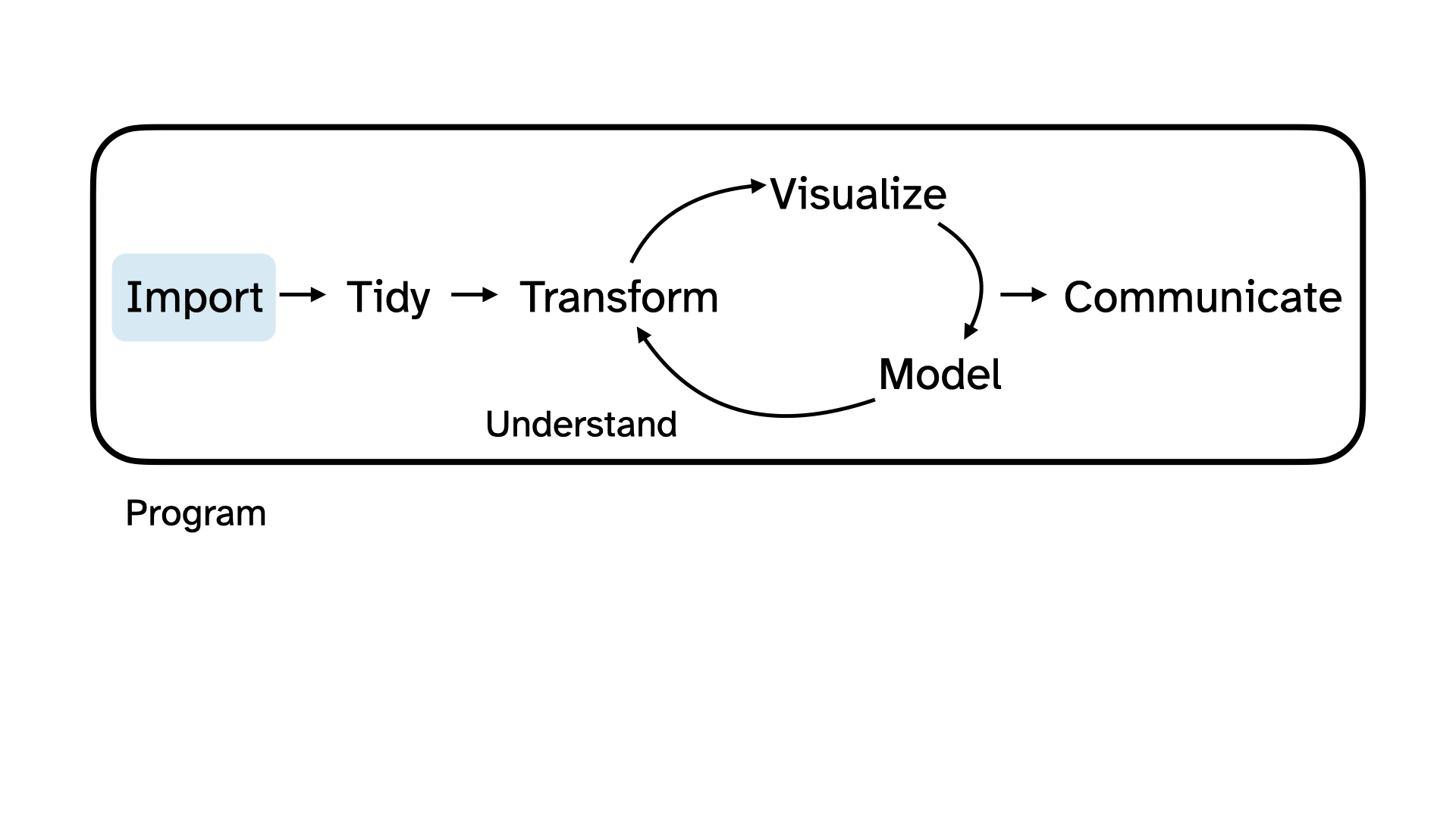
Load some packages
More on what packages are on Thursday, but in a nutshell “get your tools out of the toolbox”:
Import the data
Import the data called country-lyrics.csv in the folder called data using the read_csv() function:
country <- read_csv("data/country-lyrics.csv")Take a peek at the data
country# A tibble: 484 × 8
song artist featuring entered_top_30_in lyrics writers producer rough_order
<chr> <chr> <chr> <dbl> <chr> <chr> <chr> <dbl>
1 Wake … Craig… <NA> 2013 My fr… Josh O… Craig M… 1
2 Young… Kip M… <NA> 2013 Your … Kip Mo… Brett J… 2
3 Beat … Brett… <NA> 2013 Well … Brett … Brett E… 3
4 The H… Danie… <NA> 2013 She h… Brett … Brett J… 4
5 Every… Thomp… <NA> 2013 My mo… Keifer… RIch Re… 5
6 Goodn… Randy… <NA> 2013 Girl … Rob Ha… Derek G… 6
7 Cold … Josh … <NA> 2013 I hea… Brent … Mark Wr… 7
8 19 Yo… Dan +… <NA> 2013 It wa… Dan Sm… Dan Smy… 8
9 Hellu… Frank… <NA> 2013 Satur… Rodney… Marshal… 9
10 Chill… Cole … <NA> 2013 I got… Cole S… Jody St… 10
# ℹ 474 more rowsWhen did these songs chart?
Every song in this dataset broke into the Top 30 in some year. One way to make sense of a variable like this is to visualize it.
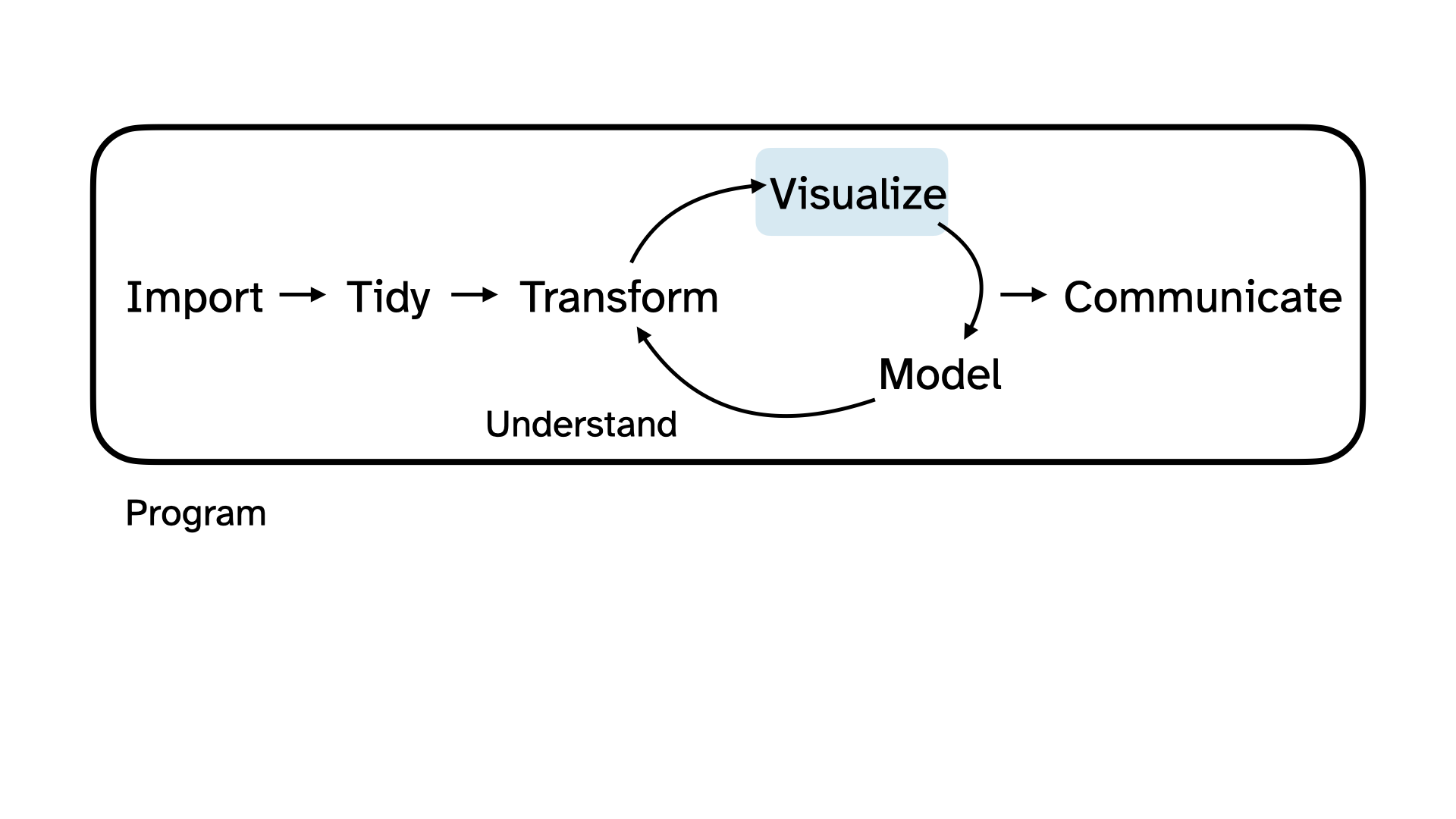
Visualize
Code
country |>
  count(entered_top_30_in) |>
  mutate(prop = n / sum(n)) |>
  ggplot(aes(x = entered_top_30_in, y = prop, group = 1)) +
  geom_point() +
  geom_line() +
  scale_y_continuous(labels = percent_format(accuracy = 1)) +
  scale_x_continuous(breaks = seq(2013, 2019, by = 1)) +
  labs(
    title = "When did these songs break into the Top 30?",
    x = NULL,
    y = NULL,
    caption = "Country songs reaching the Top 30 of Billboard's Country Airplay chart."
  ) +
  theme_minimal(base_size = 16)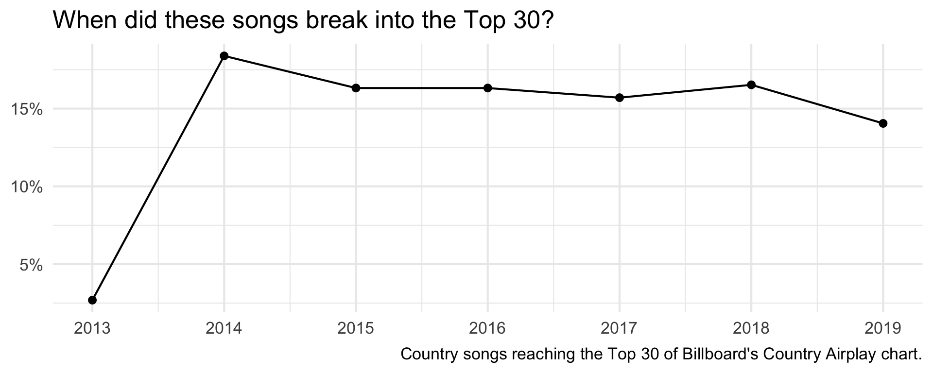
Who is on country radio?
There are 484 songs in the data, but only 121 different artists. Let’s look at the 15 with the most Top 30 hits.
Code
country |>
  count(artist, sort = TRUE) |>
  slice_head(n = 15) |>
  ggplot(aes(y = fct_reorder(artist, n), x = n, fill = n)) +
  geom_col(show.legend = FALSE) +
  labs(
    title = "Who had the most Top 30 country hits?",
    y = NULL,
    x = "Number of songs",
    caption = "Country songs reaching the Top 30 of Billboard's Country Airplay chart."
  ) +
  theme_minimal(base_size = 16)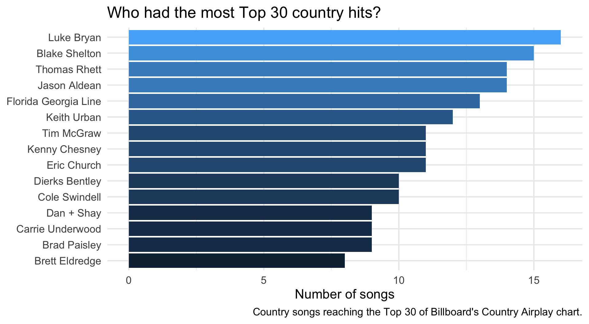
Who writes country songs?
Songs are usually written by more than one person, so the writers variable holds a whole list in a single cell:
Code
country |>
  select(song, writers)
# A tibble: 484 × 2
song writers
<chr> <chr>
1 Wake Up Lovin You Josh Osborne, Matthew Ramsey, Trevo…
2 Young Love Kip Moore, Dan Couch, Westin Davis
3 Beat of the Music Brett Eldredge, Ross Copperman, Hea…
4 The Heart of Dixie Brett James, Caitlyn Smith, Troy Ve…
5 Everything I Shouldn't Be Thinking About Keifer Thompson, Shawna Thompson, D…
6 Goodnight Kiss Rob Hatch, Jason Sellers, Randy Hou…
7 Cold Beer With Your Name On It Brent Anderson, Clint Daniels
8 19 You + Me Dan Smyers, Shay Mooney, Danny Orton
9 Helluva Life Rodney Clawson, Chris Tompkins, Jos…
10 Chillin' It Cole Swindell, Shane Minor
# ℹ 474 more rowsTidy + Transform
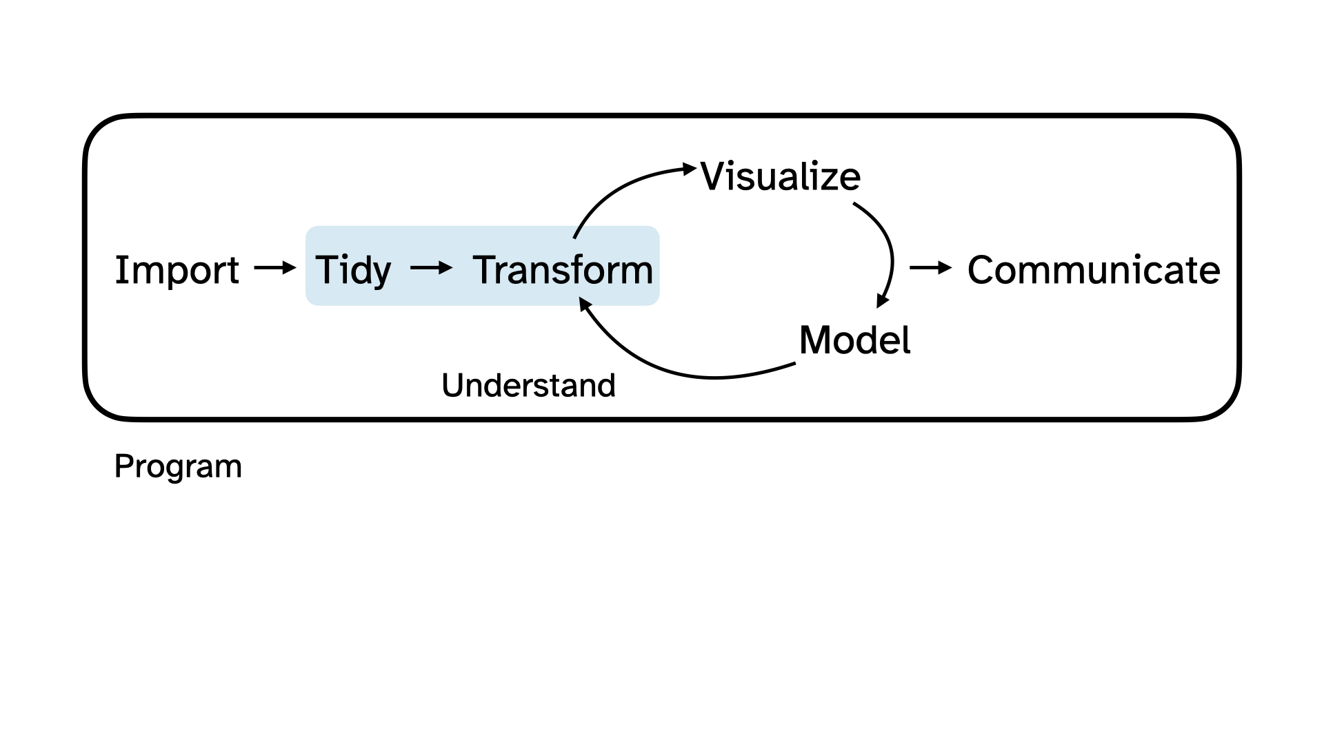
Before we can visualize this variable, we need to tidy and transform it.
Tidy + Transform
Code
country |>
  # separate into multiple rows for each writer, using comma as delimiter
  separate_longer_delim(writers, delim = ", ") |>
  count(writers, sort = TRUE)
# A tibble: 517 × 2
writers n
<chr> <int>
1 Ashley Gorley 44
2 Shane McAnally 36
3 Ross Copperman 32
4 Josh Osborne 29
5 Rhett Akins 23
6 Hillary Lindsey 18
7 Jesse Frasure 18
8 Jon Nite 17
9 Zach Crowell 16
10 Luke Laird 14
# ℹ 507 more rowsVisualize
Code
country |>
  separate_longer_delim(writers, delim = ", ") |>
  count(writers, sort = TRUE) |>
  slice_head(n = 15) |>
  ggplot(aes(y = fct_reorder(writers, n), x = n, fill = n)) +
  geom_col(show.legend = FALSE) +
  scale_fill_taylor_c(album = "Speak Now") +
  labs(
    title = "Is country radio run by a small circle of hitmakers?",
    y = NULL,
    x = "Number of songs written",
    caption = "Country songs reaching the Top 30 of Billboard's Country Airplay chart."
  ) +
  theme_minimal(base_size = 16)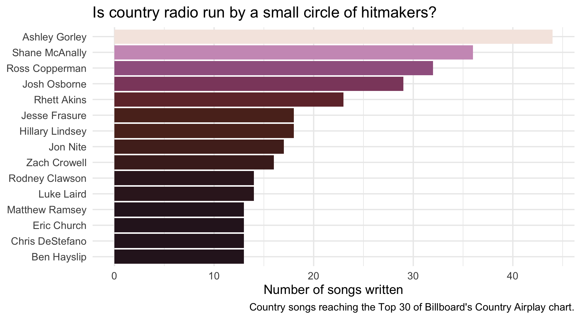
What do country songs sing about?
The lyrics variable contains the entire text of each song:
“My friends call me up ’cause they know I’m down / Take me out to paint the town and help me get over it…”
We can use text mining techniques, like tokenizing to words, to explore it.
Tidy + Transform + Summarize
Code
country |>
  select(lyrics) |>
  unnest_tokens(word, lyrics) |>
  anti_join(stop_words, by = "word") |>
  count(word, sort = TRUE) |>
  slice_head(n = 15) |>
  print(n = Inf)
# A tibble: 15 × 2
word n
<chr> <int>
1 yeah 996
2 girl 781
3 baby 749
4 love 743
5 wanna 632
6 gonna 611
7 time 502
8 night 454
9 tonight 332
10 heart 293
11 home 272
12 kiss 263
13 world 261
14 gotta 256
15 eyes 240Tokenize to bigrams
We can also tokenize to bigrams (pairs of words):
Code
country |>
  select(lyrics) |>
  unnest_tokens(bigram, lyrics, token = "ngrams", n = 2) |>
  count(bigram, sort = TRUE) |>
  slice_head(n = 8) |>
  print(n = Inf)
# A tibble: 8 × 2
bigram n
<chr> <int>
1 in the 692
2 a little 513
3 on the 413
4 and i 381
5 i know 282
6 i don't 276
7 i can 254
8 in a 249. . .
Hmm. Not very informative – these are all common words!
Drop the stop words
Let’s split each bigram in two and throw away the pairs built from common words:
Code
country |>
  select(lyrics) |>
  unnest_tokens(bigram, lyrics, token = "ngrams", n = 2) |>
  separate_wider_delim(bigram, delim = " ", names = c("word1", "word2")) |>
  anti_join(stop_words, by = join_by(word1 == word)) |>
  anti_join(stop_words, by = join_by(word2 == word)) |>
  count(word1, word2, sort = TRUE) |>
  slice_head(n = 20) |>
  print(n = Inf)
# A tibble: 20 × 3
word1 word2 n
<chr> <chr> <int>
1 yeah yeah 93
2 boo boo 81
3 ooh ooh 81
4 friday night 71
5 hey hey 45
6 tonight tonight 44
7 home home 36
8 yeah boy 33
9 saturday night 32
10 somebody's gotta 32
11 cold beer 31
12 dance floor 31
13 gonna love 31
14 country song 30
15 la la 28
16 wanna kiss 28
17 whoa whoa 28
18 da da 27
19 honky tonk 26
20 yeah baby 25Can AI help?
We could also ask a large language model to read every song and tell us what it’s about?
“What are common themes in these country song lyrics?” [Attached data file
country-lyrics.csv.] 24 August 2026. ChatGPT 5.6 Sol Light. chatgpt.com/share/e/6a8c7343-62e4-83ea-b114-715f9b847cea
Across the 484 songs in country-lyrics.csv, several recurring themes stand out:
Romantic love and attraction The dominant theme: falling in love, physical attraction, kissing, longing, and wanting to be together. Love-related language appears in roughly 94% of the songs.
Heartbreak and separation Many songs focus on breakups, regret, loneliness, missing someone, or being unable to move on. This appears in approximately 73% of the songs, often alongside love rather than separately from it.
Drinking and nightlife Beer, whiskey, bars, neon lights, and getting drunk frequently serve as settings or coping mechanisms—especially for heartbreak. Related language appears in about 60% of the songs.
Music and dancing Radios, songs, dancing, guitars, and jukeboxes are prominent. Music often brings couples together, evokes a memory, or provides the soundtrack for driving and partying. About 56% contain this imagery.
Roads, trucks, and escape Driving can represent romance, independence, returning home, or leaving a painful situation behind. Roads, trucks, and related imagery occur in approximately 55%.
Partying and carefree pleasure Friday nights, weekends, bonfires, dancing, and “good times” create an idealized space temporarily free from responsibility. This theme appears in about half the songs.
Faith, hope, and resilience References to God, prayer, heaven, belief, strength, and survival often accompany songs about hardship or gratitude. Related language occurs in approximately 43%.
Home, family, and belonging Home is both a physical place and an emotional anchor. Parents, family roots, and returning home appear in around 40% of the songs.
Rural and small-town identity Country roads, fields, porches, boots, farms, and small towns establish a distinct cultural setting and sense of authenticity. About 32% explicitly use this imagery.
Youth, memory, and nostalgia Songs frequently look back on summer, adolescence, first love, or an earlier and supposedly simpler time. Explicit nostalgic language appears in roughly 27%.
The broadest overarching theme is emotion tied to place: love, heartbreak, and personal identity are repeatedly expressed through small towns, roads, vehicles, bars, music, and home. The lyrics also contain a recurring tension between leaving and belonging—wanting to escape one’s circumstances while remaining emotionally attached to a person, hometown, or former life.
These percentages are approximate keyword-based measures, and the categories overlap: one song can simultaneously be about heartbreak, whiskey, driving, and home.
Checks and balances
Ask anyone what country songs are about and you’ll likely hear: beer, trucks, dirt roads, blue jeans, tractors.
. . .
But we have the lyrics, so we can just check:
Code
country |>
  mutate(lyrics_lower = str_to_lower(lyrics)) |>
  summarize(
    truck = mean(str_detect(lyrics_lower, "truck")),
    whiskey = mean(str_detect(lyrics_lower, "whiskey")),
    beer = mean(str_detect(lyrics_lower, "beer")),
    `dirt road` = mean(str_detect(lyrics_lower, "dirt road")),
    `blue jeans` = mean(str_detect(lyrics_lower, "blue jeans")),
    tractor = mean(str_detect(lyrics_lower, "tractor"))
  ) |>
  pivot_longer(
    everything(),
    names_to = "stereotype",
    values_to = "prop"
  ) |>
  arrange(desc(prop))
# A tibble: 6 × 2
stereotype prop
<chr> <dbl>
1 truck 0.120
2 whiskey 0.116
3 beer 0.0868
4 dirt road 0.0227
5 blue jeans 0.0227
6 tractor 0.0103Communicate
Only about 12% of these songs mention a truck, and 1% mention a tractor.
The words that actually dominate are
girl,baby,love, andnight.The stereotype is memorable, not frequent – and that difference is only visible once you look at the data.
. . .
This is what we mean by statistical thinking: a claim that “feels true” is not a finding, but you can explore and verify the claim with data and the skills you’ll learn in this course.
Course overview
Homepage
- All course materials
- Links to Canvas, GitHub, Positron containers, etc.
Course toolkit
All linked from the course website:
- GitHub organization: github.com/sta199-f26
- Positron containers: cmgr.oit.duke.edu/containers
- Communication: Ed Discussion
- Assignment submission and feedback: Gradescope
Course materials
Both textbooks are free online and linked from the course website:
- R for Data Science, 2e – Wickham, Çetinkaya-Rundel, Grolemund
- Introduction to Modern Statistics – Çetinkaya-Rundel, Hardin
Computing:
R and Positron run in containers provided by Duke OIT – nothing to install
Bring a laptop (or Chromebook) to every class, fully charged – there aren’t enough outlets in the classroom for everyone
Activities
- Introduce new content and prepare for lectures by watching the videos and completing the readings
- Attend and actively participate in lectures (and answer questions for participation credit) and labs, office hours, team meetings
- Practice applying statistical concepts and computing with application exercises during lecture
- Put together what you’ve learned to analyze real-world data
- Lab assignments
- Homework assignments
- Exams
- Term project completed in teams
Attendance and participation
Daily in lecture, via Wooclap on your laptop or phone
Tracked for credit, but not based on correctness, only participation (and often they will be questions designed to make you think that might not have a single right answer!)
There are 25 lectures this semester: participate in at least 17 for full credit
Below that, the score is prorated, e.g. participating in 15/25 lectures gives (15/25) × 5% = 3%
Application exercises
Daily-ish in lecture
Not graded, but tracked for feedback on workflow
Labs
Hands-on practice with data analysis
A single exercise per lab, graded on turning in something reasonable + correctness
Completed in-person, in lab, in teams
Teams randomized each week until project teams assigned
Developed collaboratively, but turned in individually by the end of the lab session
Two lowest scores dropped
No late work accepted
Homework
Hands-on practice with data analysis
Some questions for practice with instant feedback by AI
1-2 randomly sampled questions to be graded by humans for correctness
Can consult with course team and peers, but completed and turned in individually by 11:59 pm on Wednesdays
Lowest score dropped
Up to 3 days late (-5% per day), no late work accepted after that
One-time late penalty waiver: Can be used on any homework assignment, no questions asked, must be requested from Dr. Knox before the deadline
Turning in labs and HWs
Every assignment, same two steps:
- Push your work to the assignment’s GitHub repository
- Submit the PDF output on Gradescope
. . .
- Labs are due at the end of your lab session
- Homework is due by 11:59 pm on Wednesdays
. . .
Submit what you have even if you haven’t finished – you’ll get partial credit for your work.
Exams - structure
-
Two exams + final, all in class:
- Exam 1: Wednesday, October 7
- Exam 2: Wednesday, November 18
- Final: Thursday, December 10
-
All exams comprised of two parts:
Multiple choice questions
Short answer questions, on homework specifics (read: difficult/impossible to answer correctly without having done the homework)
Cover material from videos, readings, lectures, application exercises, homework, and labs
One sheet of notes for each exam, no larger than 8 1/2 x 11, both sides, must be prepared by you
Exams - policies
No extensions and no make-up exams.
-
With documentation (Dean’s excuse or similar):
- Miss Exam 1 or 2 → your final exam score replaces the missed score
- Miss the Final → you receive an Incomplete and take the final later
Improvement bonus: If you take all three exams, your final exam score replaces the lower of your two mid-semester exam scores – if the final score is higher.
Exam dates cannot be changed and no make-up exams will be given. If you can’t take the exams on Oct 7, Nov 18, and Dec 10, you should drop this class.
Project
Dataset of your choice, method of your choice
Teamwork
Seven milestones, interim deadlines throughout semester
Final milestone: Presentation in lab and write-up, Thursday, Nov 5
Must be in lab, in-person to present
Peer feedback between teams on presentation content; peer evaluation within teams for contribution, alongside commit history
Some lab sessions allocated to project progress
The project presentation date (Nov 5) cannot be changed, and no late work is accepted for the project. You must complete the project to pass this class.
Teams
Randomized at first for weekly labs
Then selected by you or assigned by me if you don’t express a preference for project and remaining labs
-
Expectations and roles
- Everyone is expected to contribute equal effort
- Everyone is expected to understand all code turned in
- Individual contribution evaluated by peer evaluation, commits, etc.
For the project: Peer evaluation during teamwork and after completion
Grading
| Category | Percentage |
|---|---|
| Lectures (attendance + participation) | 5% |
| HW | 5% |
| Labs | 10% |
| Project | 15% |
| Exam 1 | 20% |
| Exam 2 | 20% |
| Final | 25% |
See course syllabus for how the final letter grade will be determined.
Policies and support
Tips for success
- Prepare: Watch videos and read before class
- Engage: Attend all lectures and labs actively
- Ask questions: Use office hours and Ed Discussion forum
- Start early: Don’t procrastinate on assignments
- Stay current: Content builds progressively
Support
- Help from humans:
- Attend office hours
- Ask and answer questions on the discussion forum
- Reserve email for questions on personal matters and/or grades, and include “STA 199” in the subject line
- Extensions, accommodations, missed work, registration → course coordinator Dr. Mary Knox, mary.knox@duke.edu
- Anything else not suited to the forum → Dr. Çetinkaya-Rundel, mc301@duke.edu
- Expect a reply within 48 hours, Monday through Friday; slower over the weekend
- Read the course support page
Announcements
- Posted on Canvas (Announcements tool) and sent via email, be sure to check both regularly
- I’ll assume that you’ve read an announcement by the next “business” day
- I’ll (try my best to) send a weekly update announcement each Friday, outlining the plan for the following week and reminding you what you need to do to prepare, practice, and perform
Wrap up
Tasks due Wednesday
- Complete the getting to know you survey, then accept your GitHub organization invitation
- Read the syllabus
- Complete readings and videos for Wednesday
All linked from the course website at