x |>
  filter(x1 == "a") |>
select(x1, x2, x5)Exploratory data analysis I
Lecture 5
Warm up
While you wait: Participate 📱
Suppose you have a dataset df with 100 rows and 5 columns: x1, x2, x3, x4, and x5. x1 is a categorical variable with levels a and b. You run the following code:
The resulting data frame will have:
- 3 columns, 50 rows
- 3 columns, 100 rows
- 3 columns, can’t tell how many rows
- 5 columns, 100 rows
- 5 columns, can’t tell how many rows

Go to wooclap.com and use the code KUCTINK.
Announcements
HW 1 is due tonight at 11:59 pm:
Push all work to GitHub.
Submit a PDF of your PDF file to Gradescope and mark your pages.
Getting to know you feedback: Questions
- Is the course designed for students with no prior coding or statistics background?
- What is the balance between learning statistical concepts and programming in R? How often will students code?
- How should students use readings, videos, and other materials—and which are essential?
- What should students expect from discussion projects, collaboration, and required uploads?
- What will exams look like, and what practice or study materials will be available?
- Where can students get help, and what kinds of collaboration are appropriate?
- How does the course compare to COMPSCI 216 (Everything Data) and STA 323 (Statistical Computing)?
Getting to know you feedback: Concerns
- Dominant concern: lack of prior coding experience—especially learning R, syntax, troubleshooting, and technical tools such as Git and GitHub
- Keeping pace: falling behind or being less prepared than classmates
- Workload: time management for labs, HW, projects, and other commitments
- Assessment: format of exams, details of grading, and effective study strategies
- Smaller themes: Group-project dynamics, large-lecture setting, and confidence with math/statistical terminology
From last time
In this class, you will…
Build cakes (ggplot) 
Stack dolls (pipe |>) 
Master these constructs, and everything will be A-Ok!
Exploratory data analysis
Packages
Data: gerrymander
gerrymander <- read_csv("data/gerrymander.csv")What is gerrymandering?
Participate 📱💻
You are given a new dataset to analyze. What are some of the first things you would do to get to know the data?
Go to wooclap.com and use the code KUCTINK.
Data: gerrymander
glimpse(gerrymander)Rows: 443
Columns: 14
$ district <chr> "AK-00", "AL-01", "AL-02", "AL-03", "AL-04", "AL-05", "…
$ state_abb <chr> "AK", "AL", "AL", "AL", "AL", "AL", "AL", "AL", "AR", "…
$ state <chr> "Alaska", "Alabama", "Alabama", "Alabama", "Alabama", "…
$ house_rep_20 <chr> "Don Young", "Jerry Carl", "Barry Moore", "Mike Rogers"…
$ house_party_20 <chr> "Republican", "Republican", "Republican", "Republican",…
$ house_rep_22 <chr> "Mary Sattler Peltola", "Jerry L Carl", "Barry Moore", …
$ house_party_22 <chr> "Democrat", "Republican", "Republican", "Republican", "…
$ house_rep_24 <chr> "Nick Begich", "Barry Moore", "Shomari Figures", "Mike …
$ house_party_24 <chr> "Republican", "Republican", "Democrat", "Republican", "…
$ harris_24 <dbl> 41.41, 21.89, 53.52, 26.18, 15.96, 34.20, 29.68, 61.45,…
$ trump_24 <dbl> 54.54, 76.94, 45.31, 72.71, 83.02, 64.02, 68.47, 37.50,…
$ gerry_22 <chr> NA, "F", "F", "F", "F", "F", "F", "F", "C", "C", "C", "…
$ gerry_24 <chr> NA, "B", "B", "B", "B", "B", "B", "B", "C", "C", "C", "…
$ gerry_26 <chr> NA, "B", "B", "B", "B", "B", "B", "B", "C", "C", "C", "…. . .
How many congressional districts are there in the United States? How many rows are there in the data? Do the number of rows in the data match your expectations?
Data: gerrymander
Rows: Congressional districts in the 2020, 2022, and 2024 elections
-
Columns:
Congressional district, state abbreviation, and state name
Name and party of the House candidate who won in 2020, 2022, and 2024
2024 election: % for Harris, % for Trump
Gerrymandering score for 2022, 2024, and 2026 (A: Good, B: Better than average with some bias, C: Average, D/F: Poor)
Variable types: district
| Variable | Type |
|---|---|
district |
categorical, ID |
state_abb |
|
state |
|
house_rep_20 |
|
house_party_20 |
|
house_rep_22 |
|
house_party_22 |
|
house_rep_24 |
|
house_party_24 |
|
harris_24 |
|
trump_24 |
|
gerry_22 |
|
gerry_24 |
|
gerry_26 |
gerrymander |>
  select(district)
# A tibble: 443 × 1
district
<chr>
1 AK-00
2 AL-01
3 AL-02
4 AL-03
5 AL-04
6 AL-05
7 AL-06
8 AL-07
9 AR-01
10 AR-02
# ℹ 433 more rowsVariable types: state_abb
| Variable | Type |
|---|---|
district |
categorical, ID |
state_abb |
categorical |
state |
|
house_rep_20 |
|
house_party_20 |
|
house_rep_22 |
|
house_party_22 |
|
house_rep_24 |
|
house_party_24 |
|
harris_24 |
|
trump_24 |
|
gerry_22 |
|
gerry_24 |
|
gerry_26 |
gerrymander |>
  select(district, state_abb)
# A tibble: 443 × 2
district state_abb
<chr> <chr>
1 AK-00 AK
2 AL-01 AL
3 AL-02 AL
4 AL-03 AL
5 AL-04 AL
6 AL-05 AL
7 AL-06 AL
8 AL-07 AL
9 AR-01 AR
10 AR-02 AR
# ℹ 433 more rowsVariable types: state
| Variable | Type |
|---|---|
district |
categorical, ID |
state_abb |
categorical |
state |
categorical |
house_rep_20 |
|
house_party_20 |
|
house_rep_22 |
|
house_party_22 |
|
house_rep_24 |
|
house_party_24 |
|
harris_24 |
|
trump_24 |
|
gerry_22 |
|
gerry_24 |
|
gerry_26 |
gerrymander |>
  select(district, state)
# A tibble: 443 × 2
district state
<chr> <chr>
1 AK-00 Alaska
2 AL-01 Alabama
3 AL-02 Alabama
4 AL-03 Alabama
5 AL-04 Alabama
6 AL-05 Alabama
7 AL-06 Alabama
8 AL-07 Alabama
9 AR-01 Arkansas
10 AR-02 Arkansas
# ℹ 433 more rowsVariable types: House representatives
| Variable | Type |
|---|---|
district |
categorical, ID |
state_abb |
categorical |
state |
categorical |
house_rep_20 |
categorical, ID |
house_party_20 |
|
house_rep_22 |
categorical, ID |
house_party_22 |
|
house_rep_24 |
categorical, ID |
house_party_24 |
|
harris_24 |
|
trump_24 |
|
gerry_22 |
|
gerry_24 |
|
gerry_26 |
gerrymander |>
  select(district, starts_with("house_rep"))
# A tibble: 443 × 4
district house_rep_20 house_rep_22 house_rep_24
<chr> <chr> <chr> <chr>
1 AK-00 "Don Young" "Mary Sattler Peltola" "Nick Begic…
2 AL-01 "Jerry Carl" "Jerry L Carl" "Barry Moor…
3 AL-02 "Barry Moore" "Barry Moore" "Shomari Fi…
4 AL-03 "Mike Rogers" "Mike Rogers" "Mike Roger…
5 AL-04 "Robert B Aderholt" "Robert B Aderholt" "Robert B. …
6 AL-05 "Mo Brooks" "Dale Strong" "Dale W. St…
7 AL-06 "Gary J Palmer" "Gary J Palmer" "Gary J. Pa…
8 AL-07 "Terri A Sewell" "Terri A Sewell" "Terri A. S…
9 AR-01 "Eric A \\\"Rick\\\" Crawford" "Eric A Â\u0080\u009cRi… "Eric A. \\…
10 AR-02 "J French Hill" "J French Hill" "J. French …
# ℹ 433 more rowsVariable types: winning parties
| Variable | Type |
|---|---|
district |
categorical, ID |
state_abb |
categorical |
state |
categorical |
house_rep_20 |
categorical, ID |
house_party_20 |
categorical |
house_rep_22 |
categorical, ID |
house_party_22 |
categorical |
house_rep_24 |
categorical, ID |
house_party_24 |
categorical |
harris_24 |
|
trump_24 |
|
gerry_22 |
|
gerry_24 |
|
gerry_26 |
gerrymander |>
  select(district, starts_with("house_party"))
# A tibble: 443 × 4
district house_party_20 house_party_22 house_party_24
<chr> <chr> <chr> <chr>
1 AK-00 Republican Democrat Republican
2 AL-01 Republican Republican Republican
3 AL-02 Republican Republican Democrat
4 AL-03 Republican Republican Republican
5 AL-04 Republican Republican Republican
6 AL-05 Republican Republican Republican
7 AL-06 Republican Republican Republican
8 AL-07 Democrat Democrat Democrat
9 AR-01 Republican Republican Republican
10 AR-02 Republican Republican Republican
# ℹ 433 more rowsVariable types: harris_24 and trump_24
| Variable | Type |
|---|---|
district |
categorical, ID |
state_abb |
categorical |
state |
categorical |
house_rep_20 |
categorical, ID |
house_party_20 |
categorical |
house_rep_22 |
categorical, ID |
house_party_22 |
categorical |
house_rep_24 |
categorical, ID |
house_party_24 |
categorical |
harris_24 |
numerical, continuous |
trump_24 |
numerical, continuous |
gerry_22 |
|
gerry_24 |
|
gerry_26 |
gerrymander |>
  select(district, harris_24, trump_24)
# A tibble: 443 × 3
district harris_24 trump_24
<chr> <dbl> <dbl>
1 AK-00 41.4 54.5
2 AL-01 21.9 76.9
3 AL-02 53.5 45.3
4 AL-03 26.2 72.7
5 AL-04 16.0 83.0
6 AL-05 34.2 64.0
7 AL-06 29.7 68.5
8 AL-07 61.4 37.5
9 AR-01 26.4 71.7
10 AR-02 41.0 56.6
# ℹ 433 more rowsVariable types: Gerrymandering level
| Variable | Type |
|---|---|
district |
categorical, ID |
state_abb |
categorical |
state |
categorical |
house_rep_20 |
categorical, ID |
house_party_20 |
categorical |
house_rep_22 |
categorical, ID |
house_party_22 |
categorical |
house_rep_24 |
categorical, ID |
house_party_24 |
categorical |
harris_24 |
numerical, continuous |
trump_24 |
numerical, continuous |
gerry_22 |
categorical, ordinal |
gerry_24 |
categorical, ordinal |
gerry_26 |
categorical, ordinal |
gerrymander |>
  select(district, starts_with("gerry"))
# A tibble: 443 × 4
district gerry_22 gerry_24 gerry_26
<chr> <chr> <chr> <chr>
1 AK-00 <NA> <NA> <NA>
2 AL-01 F B B
3 AL-02 F B B
4 AL-03 F B B
5 AL-04 F B B
6 AL-05 F B B
7 AL-06 F B B
8 AL-07 F B B
9 AR-01 C C C
10 AR-02 C C C
# ℹ 433 more rowsBased on the Gerrymandering Project’s Redistricting Report Card. (A: Good, B: Better than average with some bias, C: Average, D/F: Poor)
Univariate analysis
Univariate analysis
Analyzing a single variable:
Numerical: histogram, box plot, density plot, etc.
Categorical: bar plot, pie chart, etc.
Focus: 2024 Elections
Histogram - Step 1
ggplot(gerrymander_24)
Histogram - Step 2
Histogram - Step 3
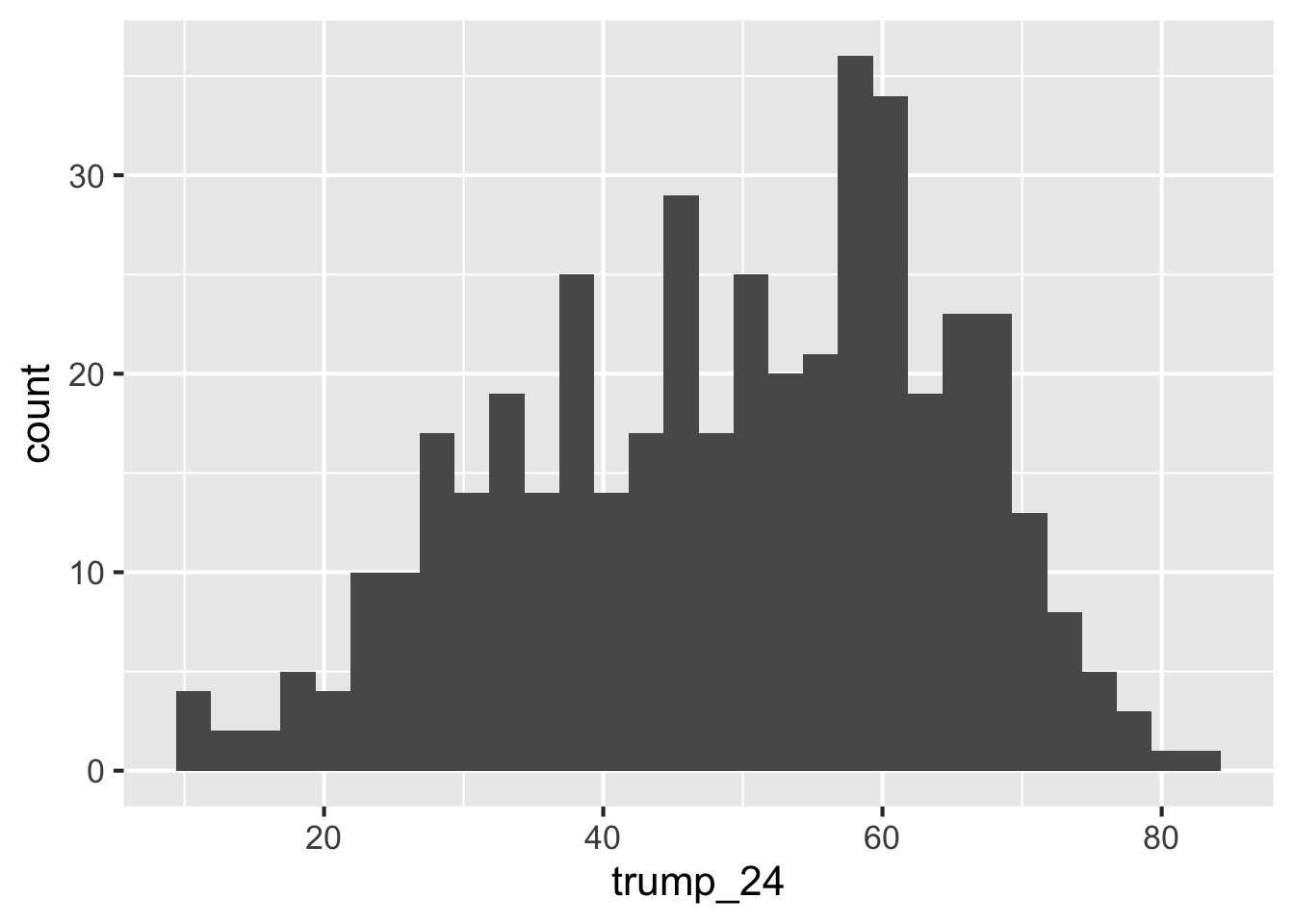
Participate 📱💻
Which of the following has the most appropriate binwidth for visualizing the distribution of trump_24?
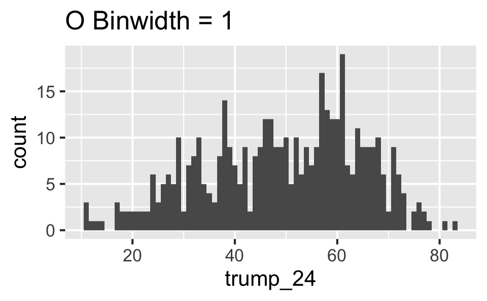
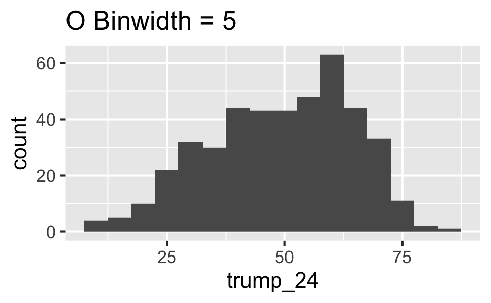
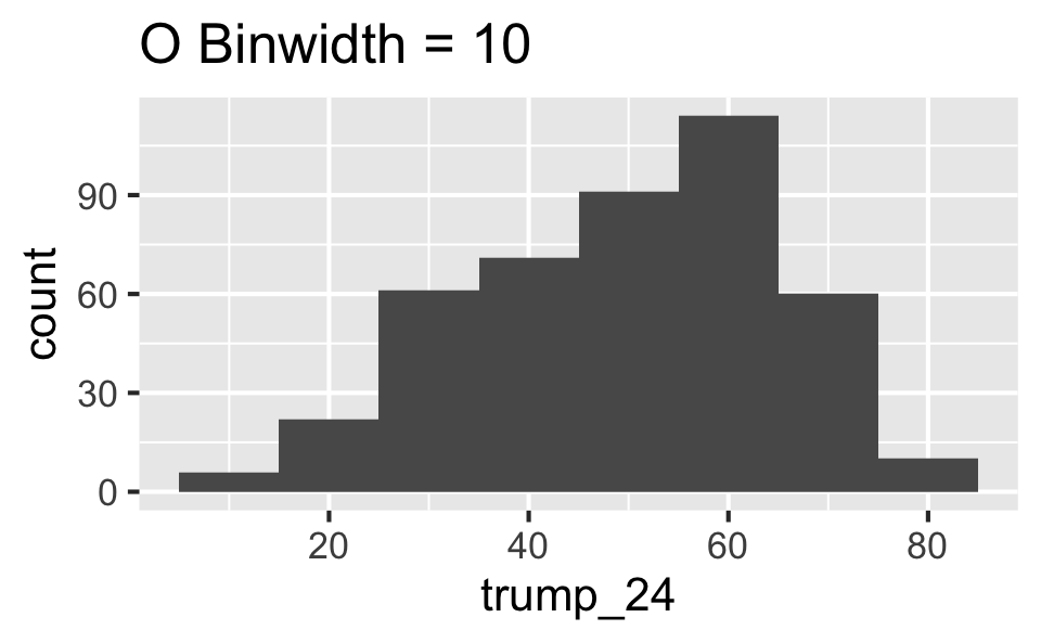
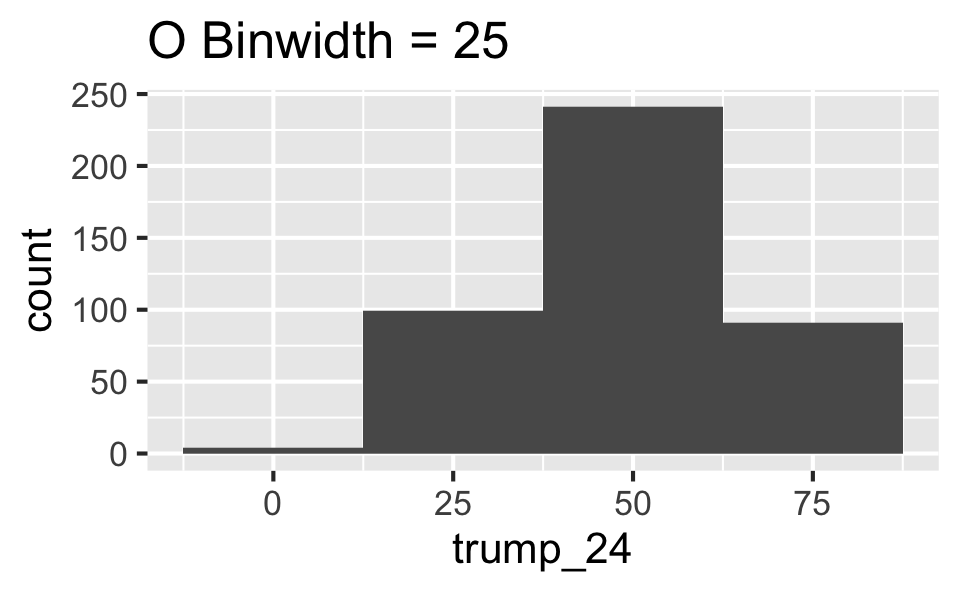
Go to wooclap.com and use the code KUCTINK.
Histogram - Step 4
Histogram - Step 5
Box plot - Step 1
ggplot(gerrymander_24)
Box plot - Step 2
Box plot - Step 3
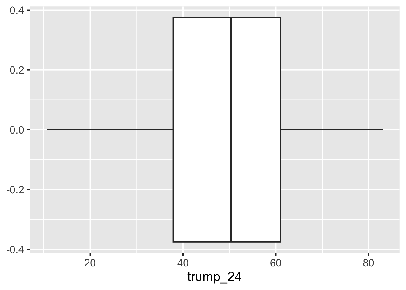
Box plot - Alternative Step 2 + 3
ggplot(gerrymander_24, aes(y = trump_24)) +
  geom_boxplot()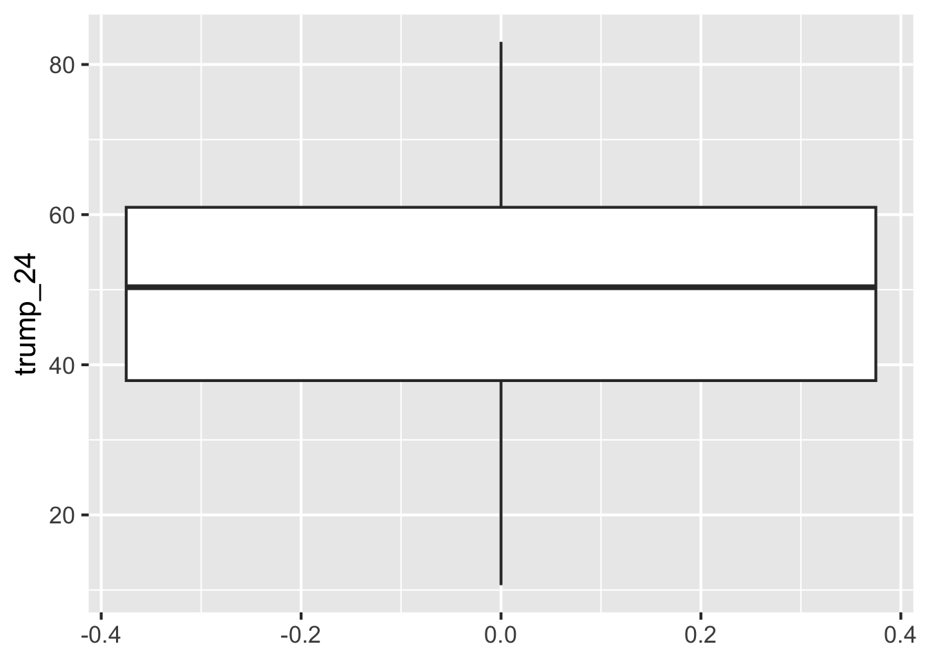
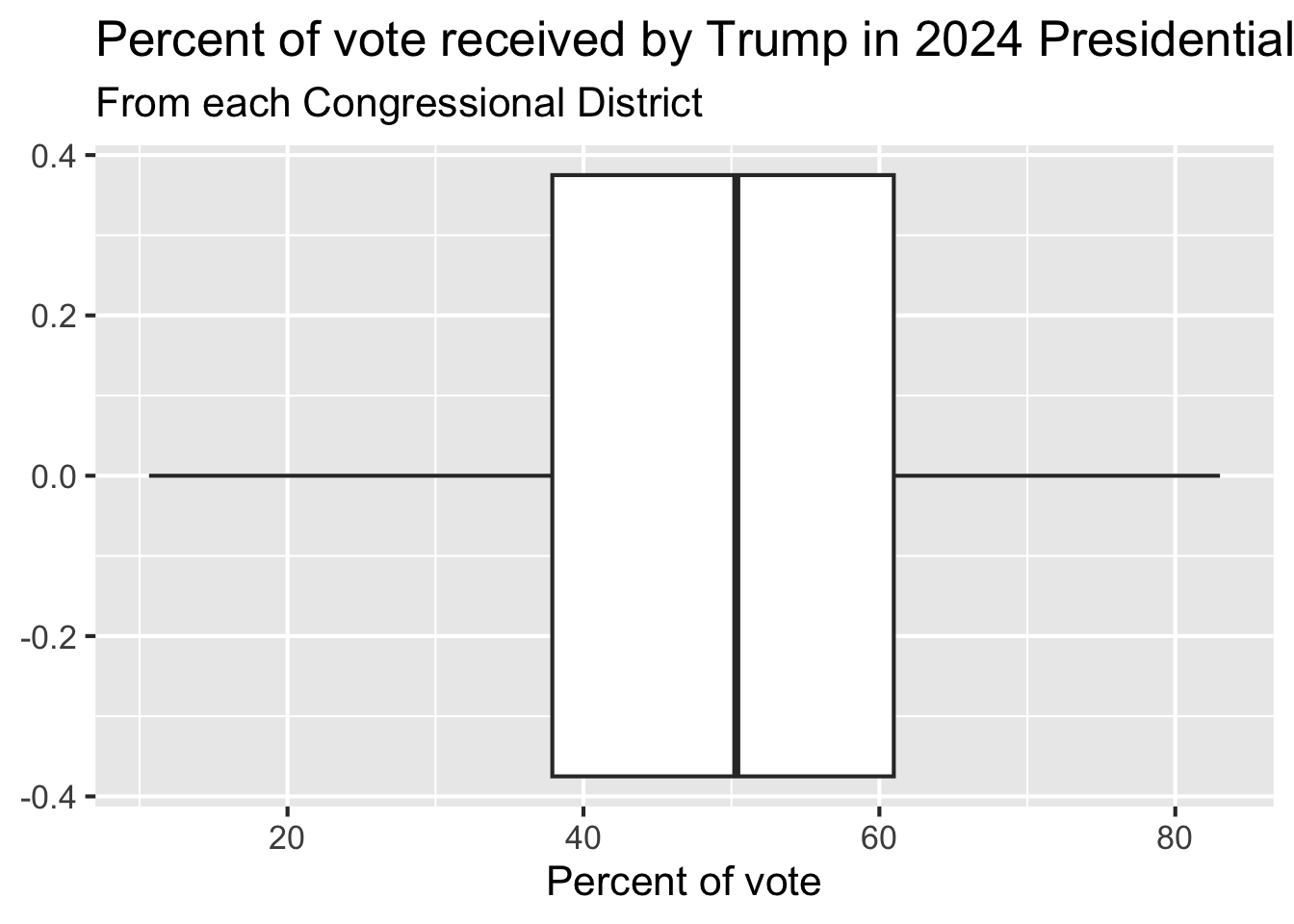
Box plot - Step 4
Density plot - Step 1
ggplot(gerrymander_24)
Density plot - Step 2
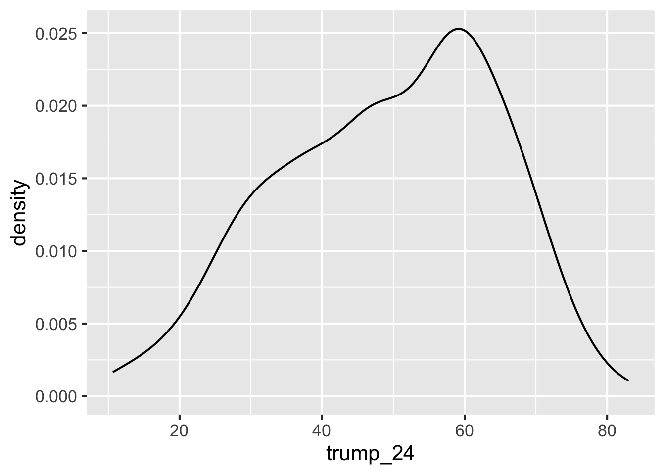
Density plot - Step 3
Density plot - Step 4
ggplot(gerrymander_24, aes(x = trump_24)) +
  geom_density(color = "firebrick")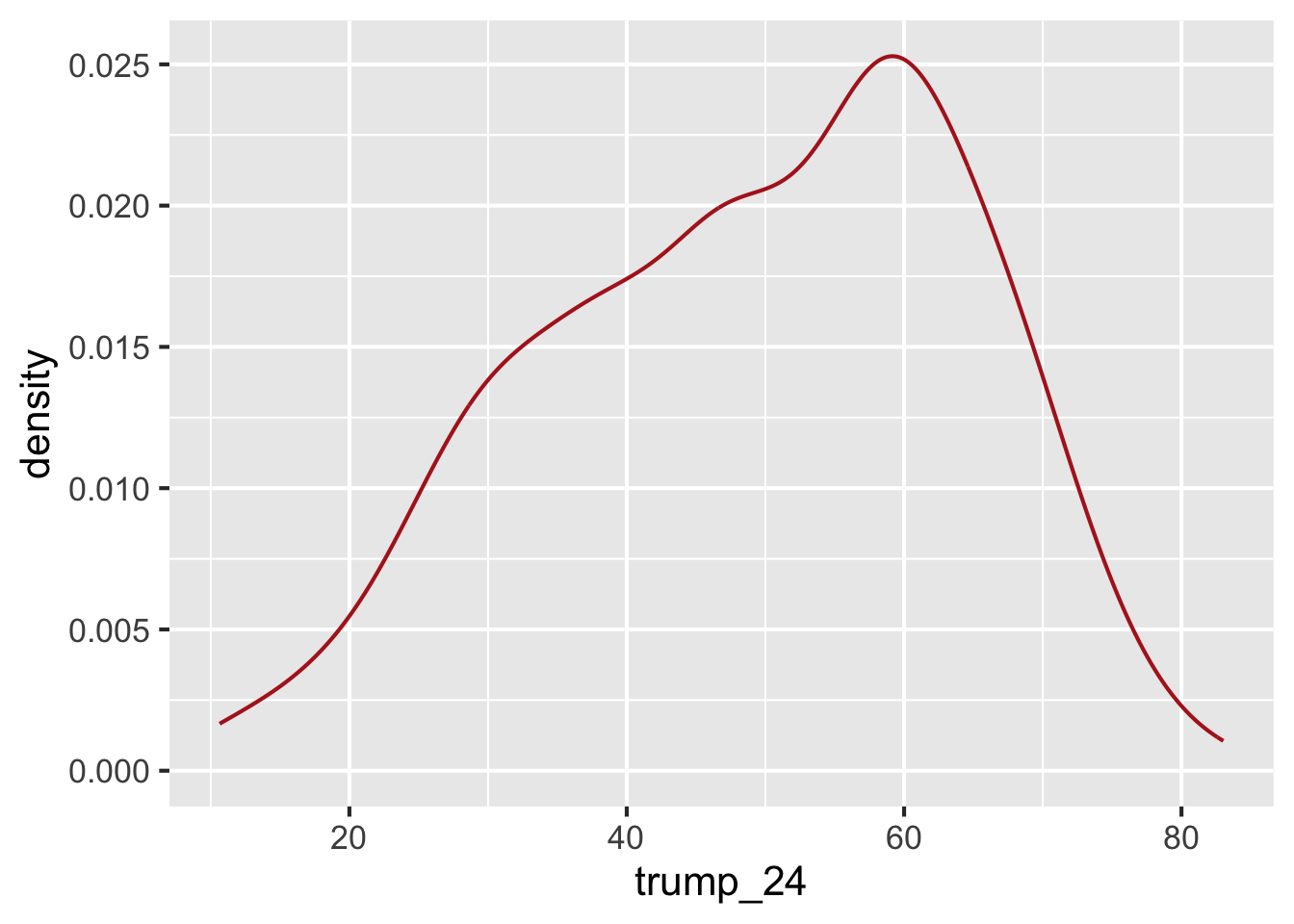
Density plot - Step 5
ggplot(gerrymander_24, aes(x = trump_24)) +
  geom_density(color = "firebrick", fill = "firebrick1")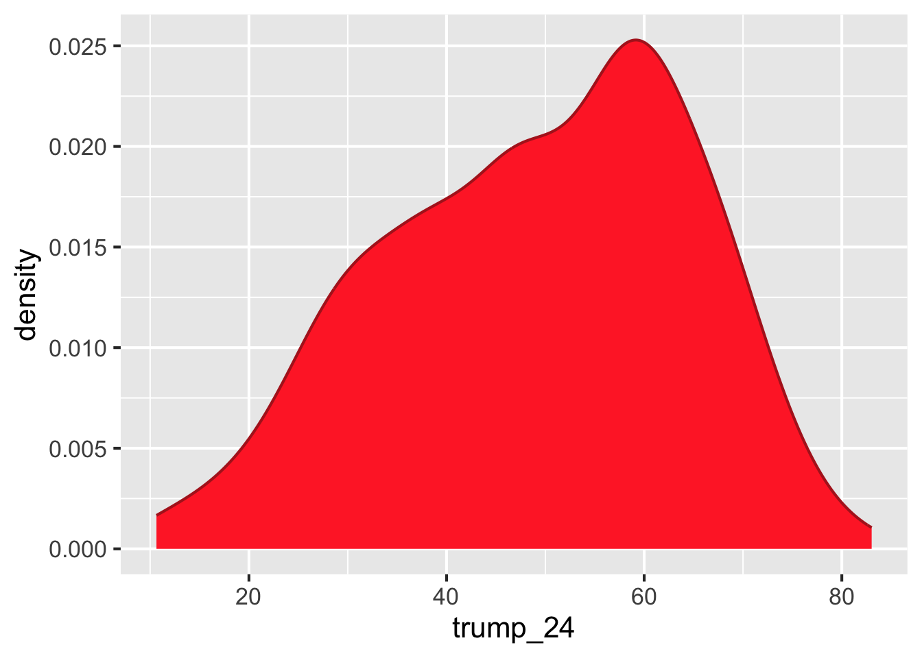
Density plot - Step 6
ggplot(gerrymander_24, aes(x = trump_24)) +
  geom_density(color = "firebrick", fill = "firebrick1", alpha = 0.5)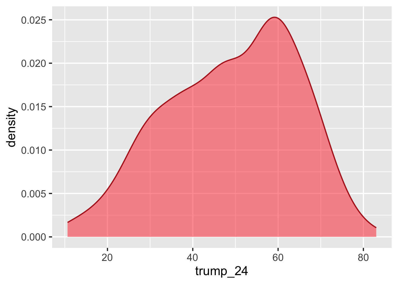
Density plot - Step 7
ggplot(gerrymander_24, aes(x = trump_24)) +
  geom_density(
    color = "firebrick",
    fill = "firebrick1",
    alpha = 0.5,
    linewidth = 1
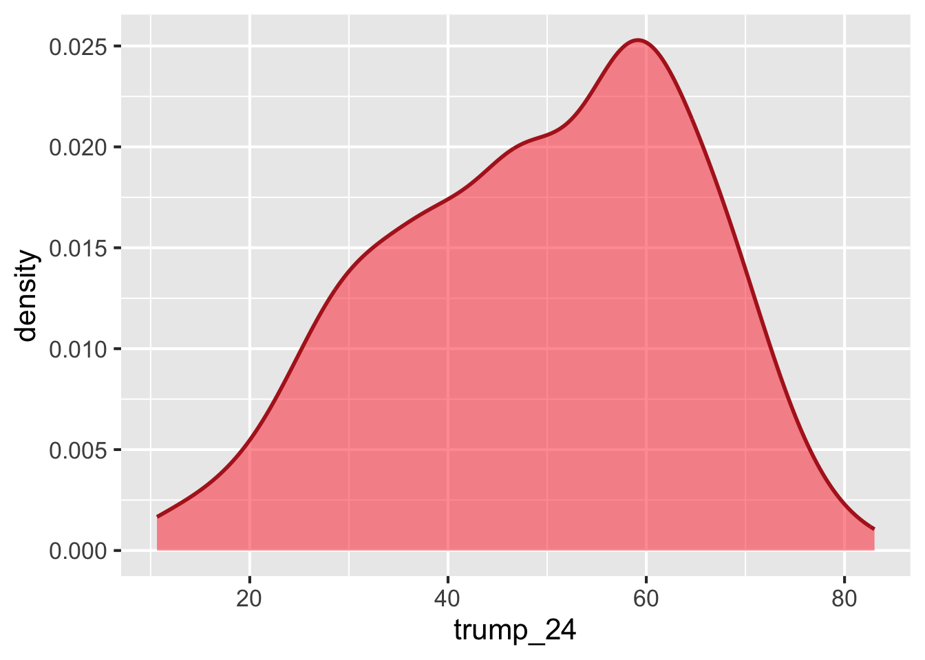
  )
Density plot - Step 8
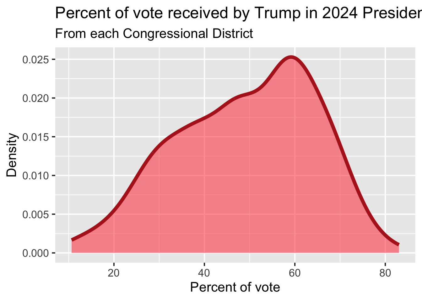
Summary statistics
gerrymander_24 |>
  summarize(
    mean = mean(trump_24),
    sd = sd(trump_24),
    min = min(trump_24),
    q25 = quantile(trump_24, 0.25),
    median = median(trump_24),
    q75 = quantile(trump_24, 0.75),
    max = max(trump_24),
  )
# A tibble: 1 × 7
mean sd min q25 median q75 max
<dbl> <dbl> <dbl> <dbl> <dbl> <dbl> <dbl>
1 49.2 15.2 10.6 37.9 50.3 61.0 83.0Distribution of votes for Trump in the 2024 election
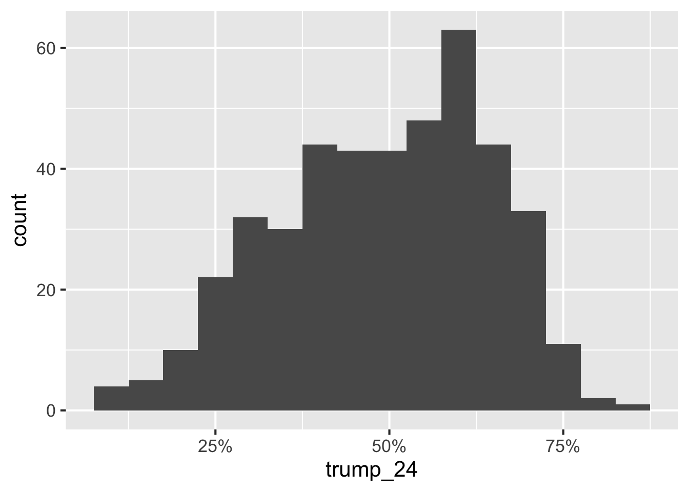
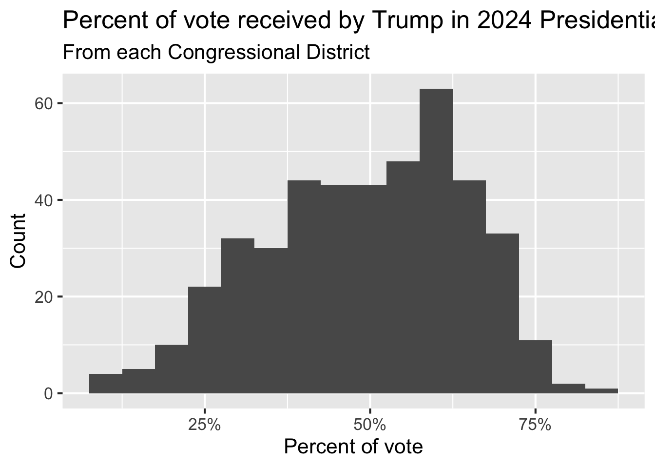
Describe the distribution of percent of vote received by Trump in 2024 Presidential Election from Congressional Districts.
Shape: The distribution of votes for Trump in the 2024 election from Congressional Districts is unimodal and left-skewed.
Center: The percent of vote received by Trump in the 2024 Presidential Election from a typical Congressional Districts is 50.3%.
Spread: In the middle 50% of Congressional Districts, 37.9% to 61% of voters voted for Trump in the 2024 Presidential Election.
Unusual observations: -
Bivariate analysis
Bivariate analysis
Analyzing the relationship between two variables:
Numerical + numerical: scatterplot
Numerical + categorical: side-by-side box plots, violin plots, etc.
Categorical + categorical: stacked bar plots
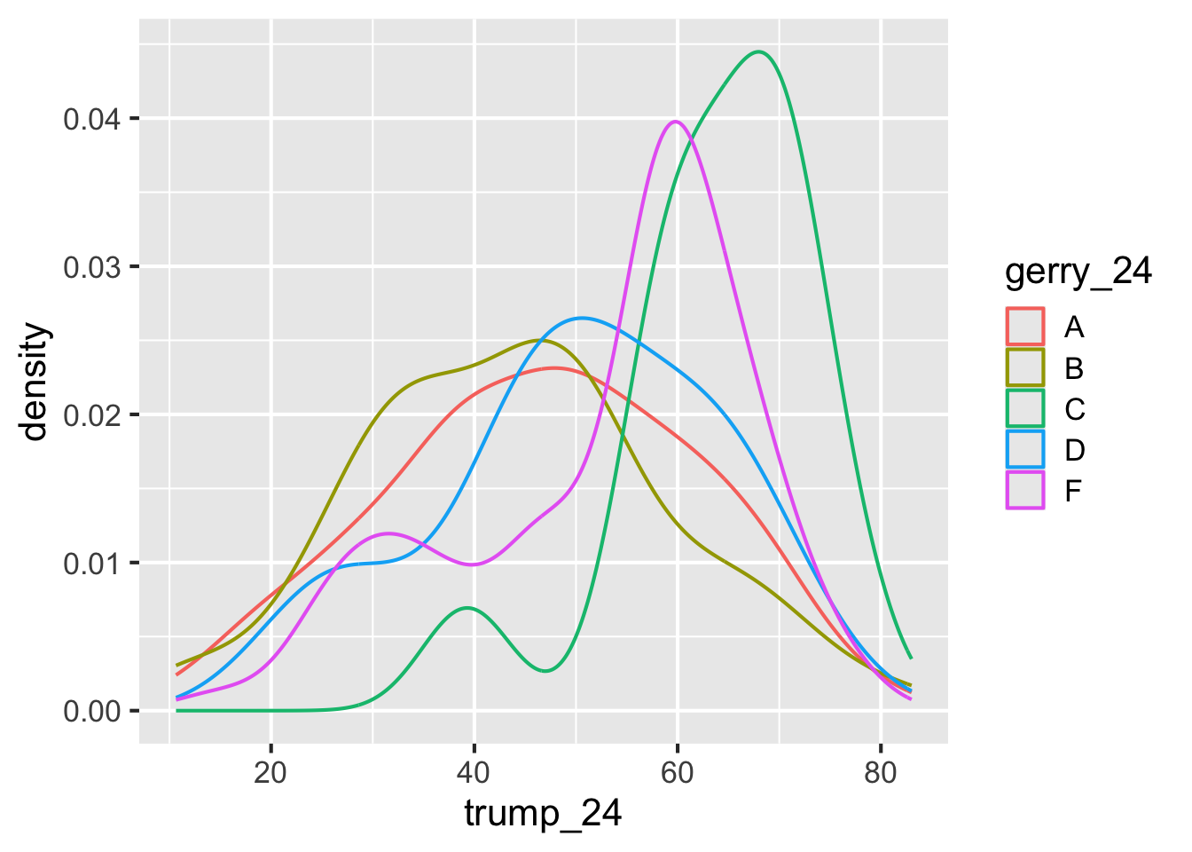
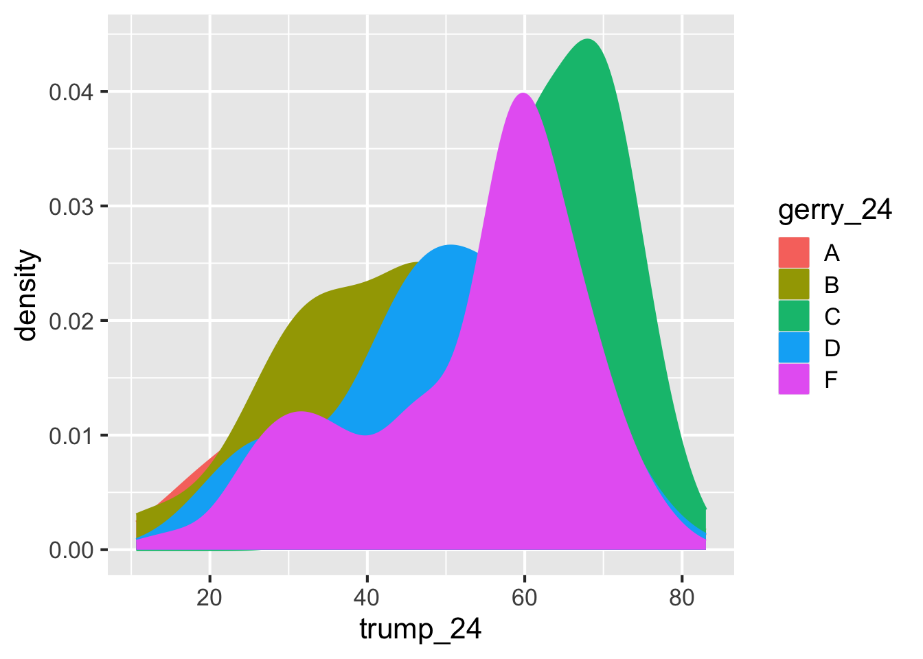
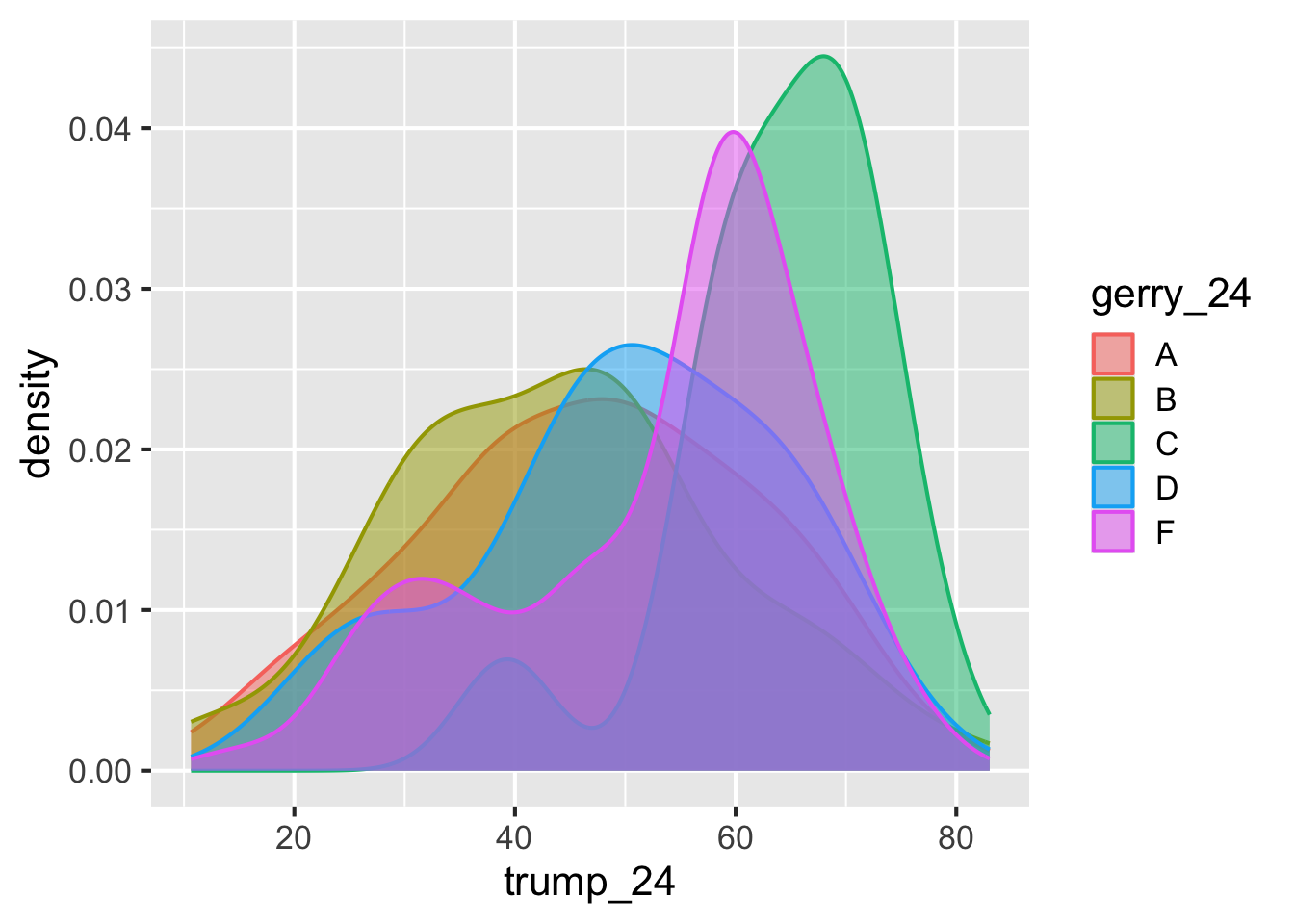
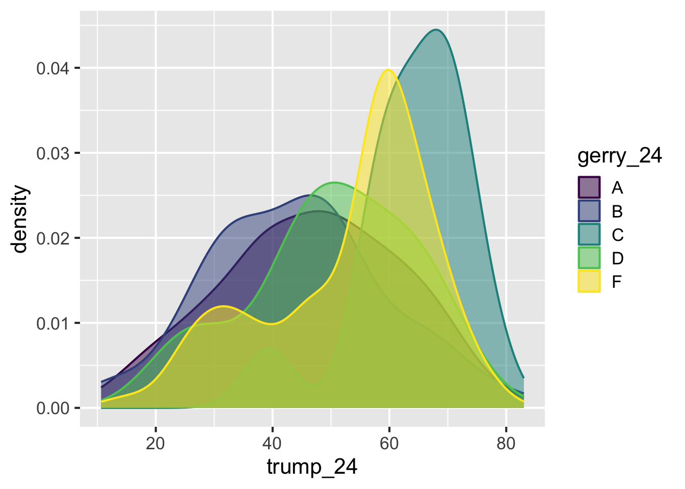
Using an aesthetic (e.g., fill, color, shape, etc.) or facets to represent the second variable in any plot
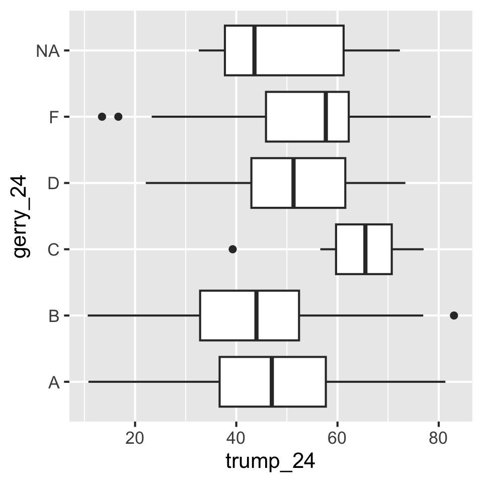
Side-by-side box plots
Participate 📱💻
What goes in the [blank] in the code below to do the following step for each level of gerry_24?
Go to wooclap.com and use the code KUCTINK.
Grouped summary statistics
gerrymander_24 |>
  group_by(gerry_24) |>
  summarize(
    min = min(trump_24),
    q25 = quantile(trump_24, 0.25),
    median = median(trump_24),
    q75 = quantile(trump_24, 0.75),
    max = max(trump_24),
  )
# A tibble: 6 × 6
gerry_24 min q25 median q75 max
<chr> <dbl> <dbl> <dbl> <dbl> <dbl>
1 A 10.8 36.7 47.0 57.7 81.3
2 B 10.6 32.8 44.0 52.4 83.0
3 C 39.3 59.7 65.5 70.7 77.0
4 D 22.1 43.0 51.3 61.5 73.4
5 F 13.5 45.9 57.7 62.2 78.4
6 <NA> 32.6 37.8 43.6 61.2 72.3
NA for gerrymandering?
gerrymander_24 |>
  filter(is.na(gerry_24)) |>
  select(district, starts_with("state"), starts_with("gerry"))
# A tibble: 10 × 6
district state_abb state gerry_22 gerry_24 gerry_26
<chr> <chr> <chr> <chr> <chr> <chr>
1 AK-00 AK Alaska <NA> <NA> <NA>
2 DE-00 DE Delaware <NA> <NA> <NA>
3 HI-01 HI Hawaii <NA> <NA> <NA>
4 HI-02 HI Hawaii <NA> <NA> <NA>
5 ND-00 ND North Dakota <NA> <NA> <NA>
6 RI-01 RI Rhode Island <NA> <NA> <NA>
7 RI-02 RI Rhode Island <NA> <NA> <NA>
8 SD-00 SD South Dakota <NA> <NA> <NA>
9 VT-00 VT Vermont <NA> <NA> <NA>
10 WY-00 WY Wyoming <NA> <NA> <NA>