Linear regression with outliers and categorical predictors
Lecture 16
Author
Affiliation
Prof. Mine Çetinkaya-Rundel
Duke University STA 199 - Fall 2026
Published
October 26, 2026
Warm-up
While you wait: Participate 📱💻
In the previous class, we used food-insecurity prevalence to predict mental-distress prevalence. Durham County had a residual of -2.60 percentage points.
What should progress on projects look like nowadays?
Schedule meetings (at least one this week and at least two next week)
This week:
Outline your presentation and start drafting slides and discussing who will present which slide (each team member must speak during the presentation)
Start drafting your writeup – you can structure it as the words you will say in your presentation (i.e., your script)
Next week: Make sure at least one meeting is dedicated to practicing your presentation and timing yourself
After next week: Write the reflection portion of your writeup
From last time
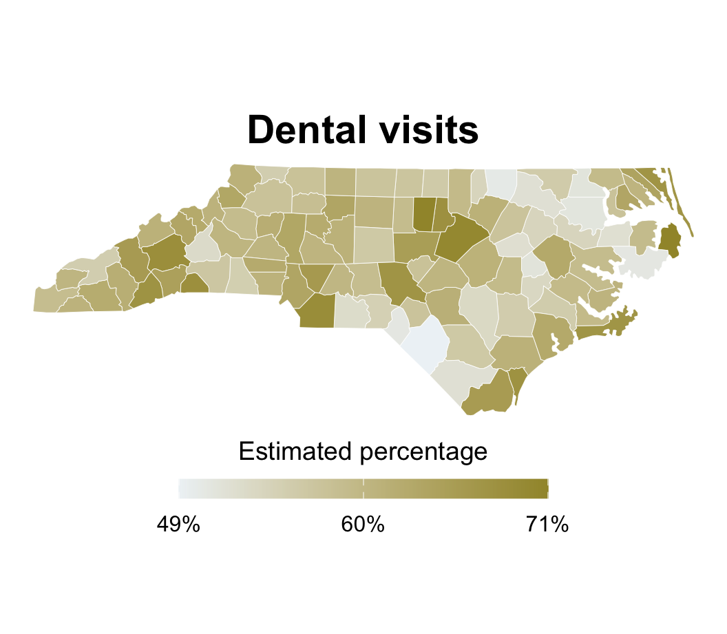
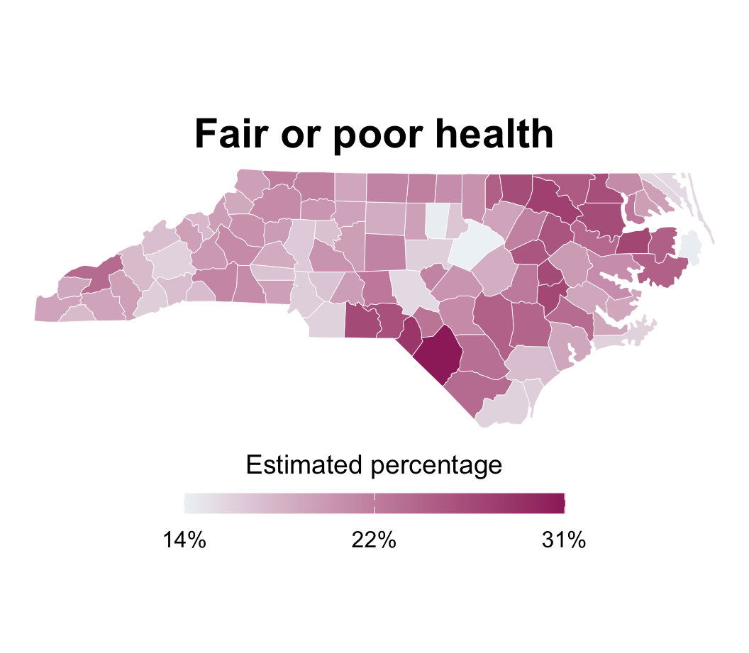
Dental visits and health
Application exercise
Go to your ae project in Positron.
If you haven’t yet done so, make sure all of your changes up to this point are committed and pushed, i.e., there’s nothing left in your source control pane.
If you haven’t yet done so, pull to get today’s application exercise file: ae-09-nc-places-model.qmd.
Work through the application exercise in class, and render, commit, and push your edits by the end of class.
Evaluating fit
Is linear model appropriate?
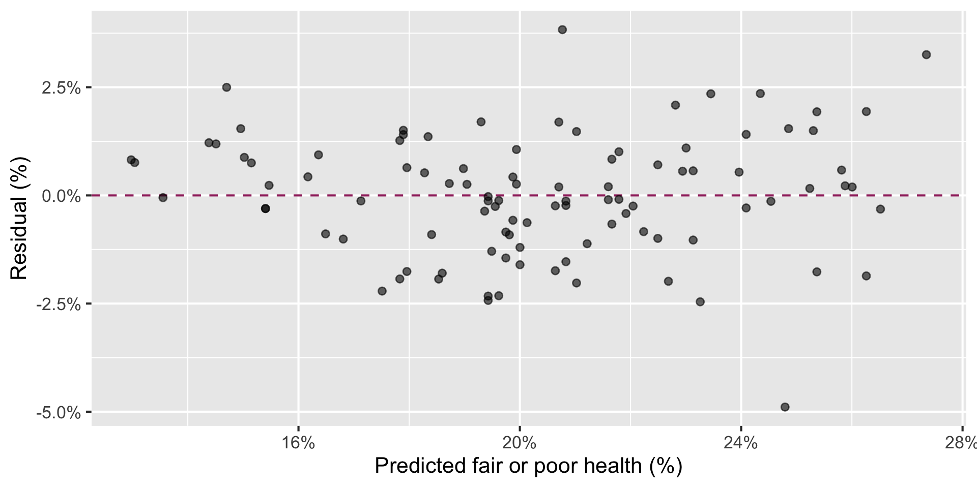
In the residuals vs. fitted (predicted) plot, we look for a horizontal band of points with no clear pattern.
Code
health_dental_fit<-linear_reg()|>fit(fair_or_poor_health~dental_visit, data =nc_places)health_dental_aug<-augment(health_dental_fit, new_data =nc_places)ggplot(health_dental_aug,aes(x =.pred, y =.resid))+geom_hline( yintercept =0, color ="#9E2C6A", linetype ="dashed")+geom_point(alpha =0.6)+scale_x_continuous(labels =label_percent(scale =1))+scale_y_continuous(labels =label_percent(scale =1))+labs( x ="Predicted fair or poor health (%)", y ="Residual (%)")
Does the model do a good job explaining the variability in the outcome?
The model (dental visits) explains 85% of the variability in fair or poor health percentage in NC counties.
What observations stand out from the main cloud of points? In what way do they stand out?
Outliers in regression
An outlier is a point—or group of points—that stands out from the rest of the data.
A leverage point is horizontally far from the center of the cloud. It has the potential to pull harder on the fitted line.
An influential point actually changes the slope or position of the fitted line substantially.
Important
These categories can overlap: a point can be an outlier, a leverage point, and an influential point.
Three counties to investigate
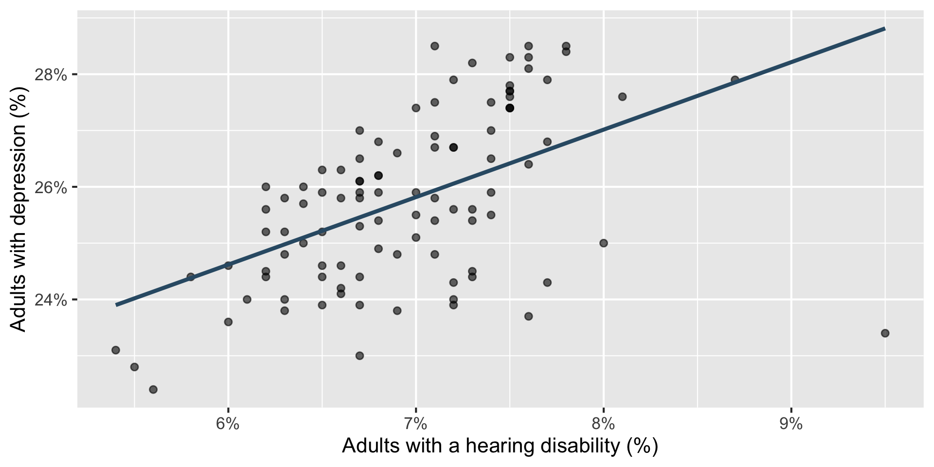
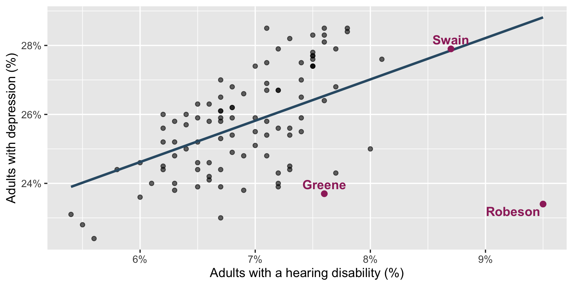
How would you classify Greene, Swain, and Robeson counties?
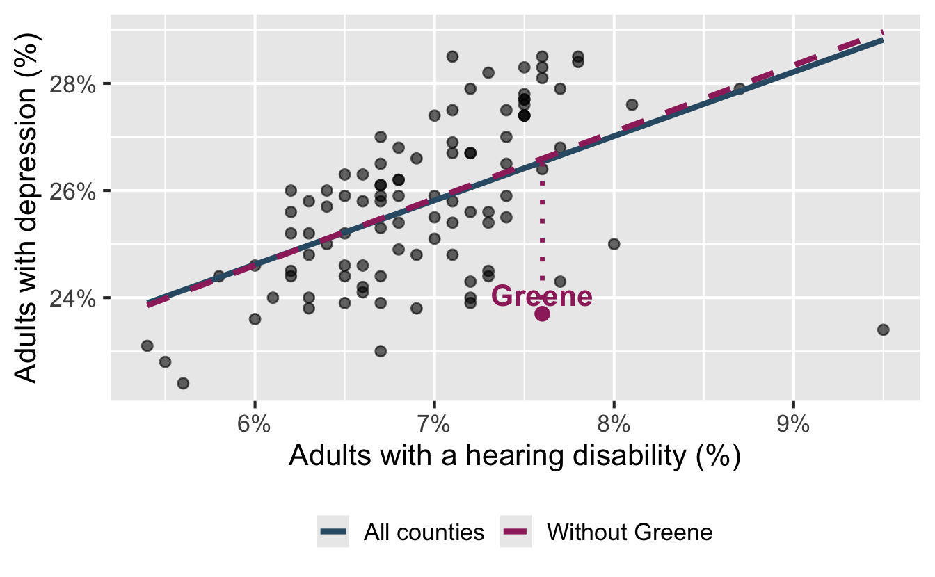
Potential outlier: Greene County
Code
greene<-hearing_depression_aug|>filter(county=="Greene")ggplot(nc_places,aes(x =hearing_disability, y =depression))+geom_point(alpha =0.6)+geom_smooth(aes(color ="All counties", linetype ="All counties"), method ="lm", se =FALSE)+geom_smooth( data =nc_places|>filter(county!="Greene"),aes(color ="Without Greene", linetype ="Without Greene"), method ="lm", se =FALSE)+scale_color_manual( values =c("All counties"="#325b74","Without Greene"="#9E2C6A"))+scale_linetype_manual( values =c("All counties"="solid","Without Greene"="dashed"))+scale_x_continuous(labels =label_percent(scale =1))+scale_y_continuous(labels =label_percent(scale =1))+labs( x ="Adults with a hearing disability (%)", y ="Adults with depression (%)", color =NULL, linetype =NULL)+geom_segment( data =greene,aes( x =hearing_disability, xend =hearing_disability, y =.pred, yend =depression), color ="#9E2C6A", linewidth =1.2, linetype ="dotted")+geom_point(data =greene, color ="#9E2C6A", size =3)+geom_text( data =greene,aes(label =county), color ="#9E2C6A", fontface ="bold", nudge_y =0.35)+theme(legend.position ="bottom")
Greene is vertically far below the fitted line.
Its hearing-disability prevalence is near the center of the observed values.
Removing Greene barely changes the slope.
Greene County is a potential outlier in this relationship, but not a leverage or influential point.
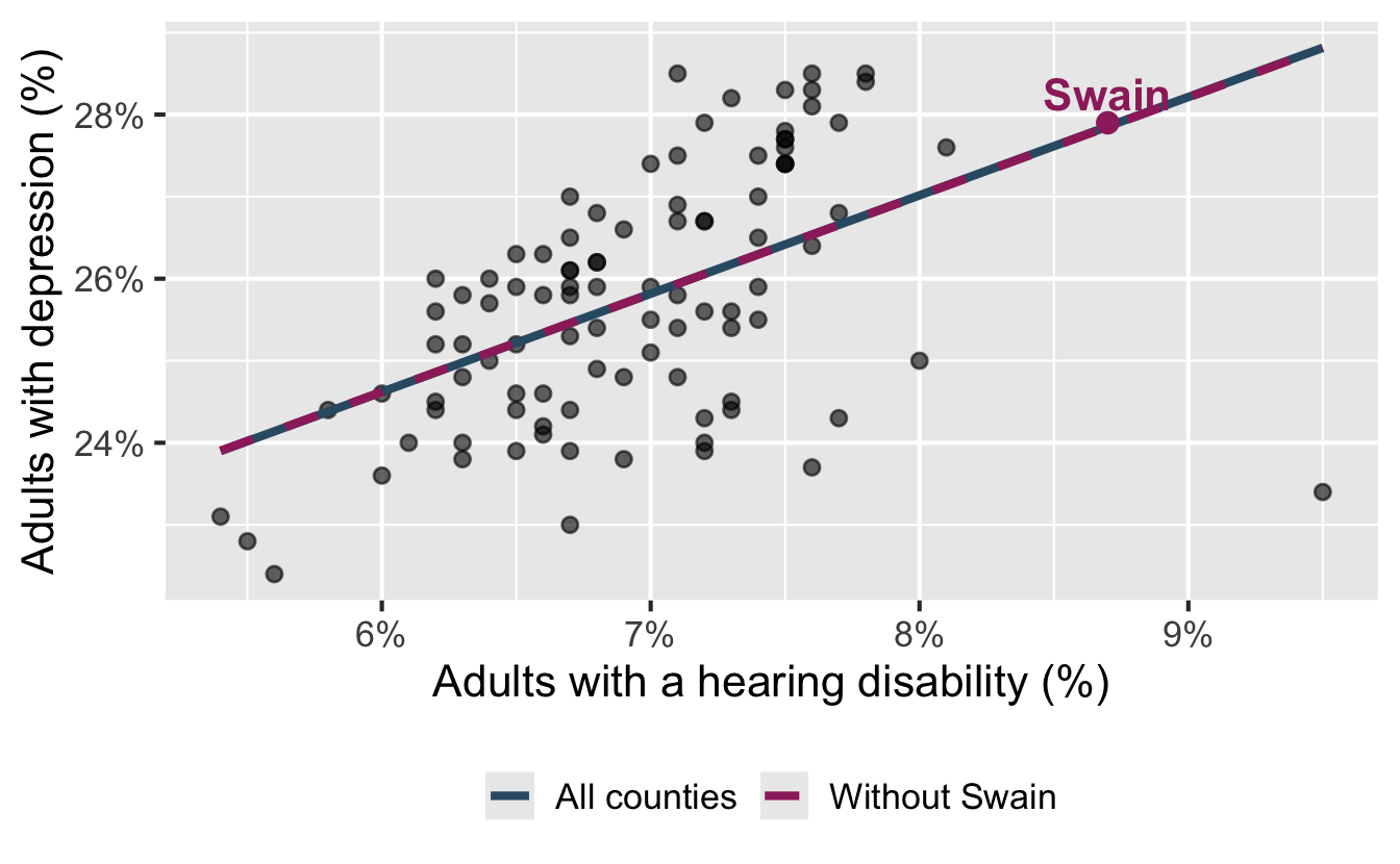
Leverage point: Swain County
Code
swain<-hearing_depression_aug|>filter(county=="Swain")ggplot(nc_places,aes(x =hearing_disability, y =depression))+geom_point(alpha =0.6)+geom_smooth(aes(color ="All counties", linetype ="All counties"), method ="lm", se =FALSE)+geom_smooth( data =nc_places|>filter(county!="Swain"),aes(color ="Without Swain", linetype ="Without Swain"), method ="lm", se =FALSE)+scale_color_manual( values =c("All counties"="#325b74","Without Swain"="#9E2C6A"))+scale_linetype_manual( values =c("All counties"="solid","Without Swain"="dashed"))+scale_x_continuous(labels =label_percent(scale =1))+scale_y_continuous(labels =label_percent(scale =1))+labs( x ="Adults with a hearing disability (%)", y ="Adults with depression (%)", color =NULL, linetype =NULL)+geom_segment( data =swain,aes( x =hearing_disability, xend =hearing_disability, y =.pred, yend =depression), color ="#9E2C6A", linewidth =1.2, linetype ="dotted")+geom_point(data =swain, color ="#9E2C6A", size =3)+geom_text( data =swain,aes(label =county), color ="#9E2C6A", fontface ="bold", nudge_y =0.35)+theme(legend.position ="bottom")
Swain is horizontally far from the center of the cloud.
It lies almost exactly on the fitted line: its residual is tiny.
Removing Swain barely changes the fitted line.
Swain County is a high-leverage point in this relationship, but not an outlier or influential point.
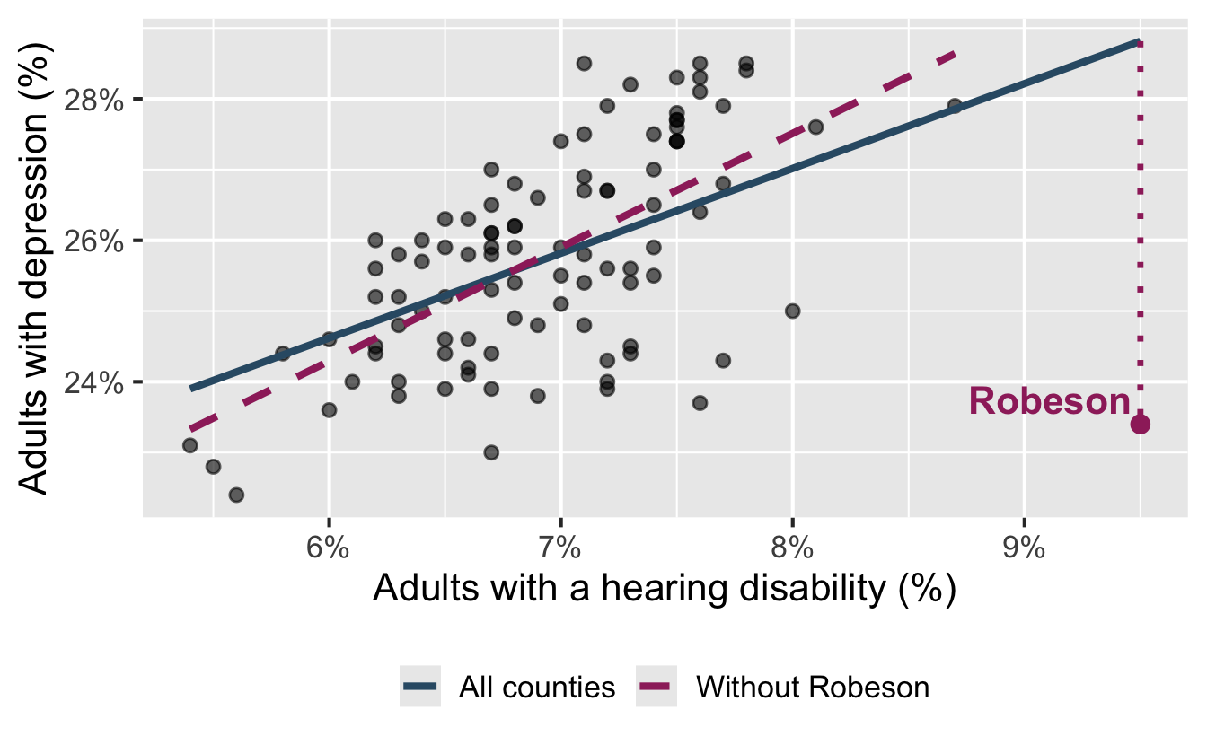
Influential point: Robeson County
Code
robeson<-hearing_depression_aug|>filter(county=="Robeson")ggplot(nc_places,aes(x =hearing_disability, y =depression))+geom_point(alpha =0.6)+geom_smooth(aes(color ="All counties", linetype ="All counties"), method ="lm", se =FALSE)+geom_smooth( data =nc_places|>filter(county!="Robeson"),aes(color ="Without Robeson", linetype ="Without Robeson"), method ="lm", se =FALSE)+scale_color_manual( values =c("All counties"="#325b74","Without Robeson"="#9E2C6A"))+scale_linetype_manual( values =c("All counties"="solid","Without Robeson"="dashed"))+scale_x_continuous(labels =label_percent(scale =1))+scale_y_continuous(labels =label_percent(scale =1))+labs( x ="Adults with a hearing disability (%)", y ="Adults with depression (%)", color =NULL, linetype =NULL)+geom_segment( data =robeson,aes( x =hearing_disability, xend =hearing_disability, y =.pred, yend =depression), color ="#9E2C6A", linewidth =1.2, linetype ="dotted")+geom_point(data =robeson, color ="#9E2C6A", size =3)+geom_text( data =robeson,aes(label =county), color ="#9E2C6A", fontface ="bold", nudge_y =0.35, hjust =1.05)+theme(legend.position ="bottom")
Robeson County is an influential point with high-leverage.
Robeson is horizontally far from the center of the cloud.
It also falls far below the fitted relationship: its residual has a high magnitude compared to other counties in the data.
This combination pulls the right side of the fitted line downward – the slope of the model is 1.199 with all counties and 1.609 without Robeson County.
Working with outliers
Investigate why the observation is unusual:
Is it a data or measurement error?
Is it a genuine but exceptional case?
Does it reveal a subgroup or a missing variable?
. . .
Fit the model with and without the observation and compare the results.
. . .
Do not remove an outlier solely because it is unusual. Report and justify any decision to exclude data.
Categorical predictor
Development tiers
The North Carolina Department of Commerce ranks all 100 counties by economic well-being each year. The tiers are used in state programs that aim to encourage economic activity in less prosperous areas.
Tier 1: 40 most economically distressed counties
Tier 2: next 40 counties
Tier 3: 20 least economically distressed counties
The ranking combines four equally weighted measures: unemployment, median household income, 36-month population growth, and adjusted property tax base per capita.
predictor: county development tier (categorical; Tier 1 is most economically distressed and Tier 3 is least economically distressed)
Visualize
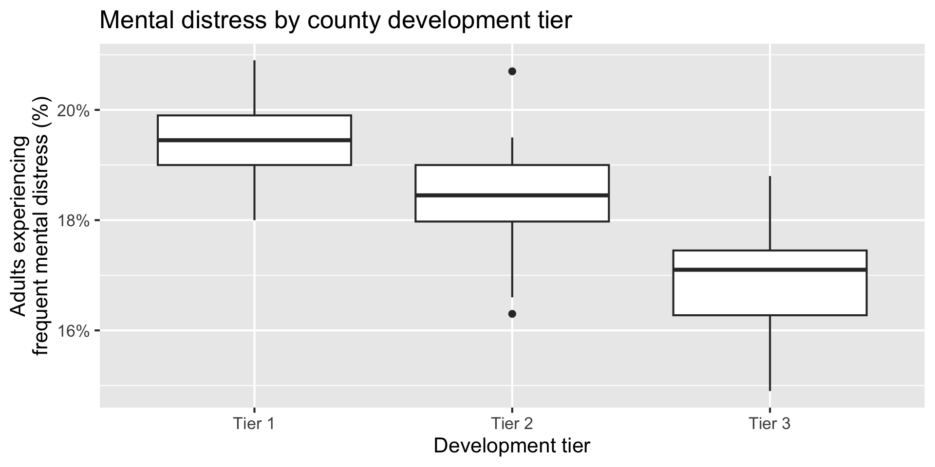
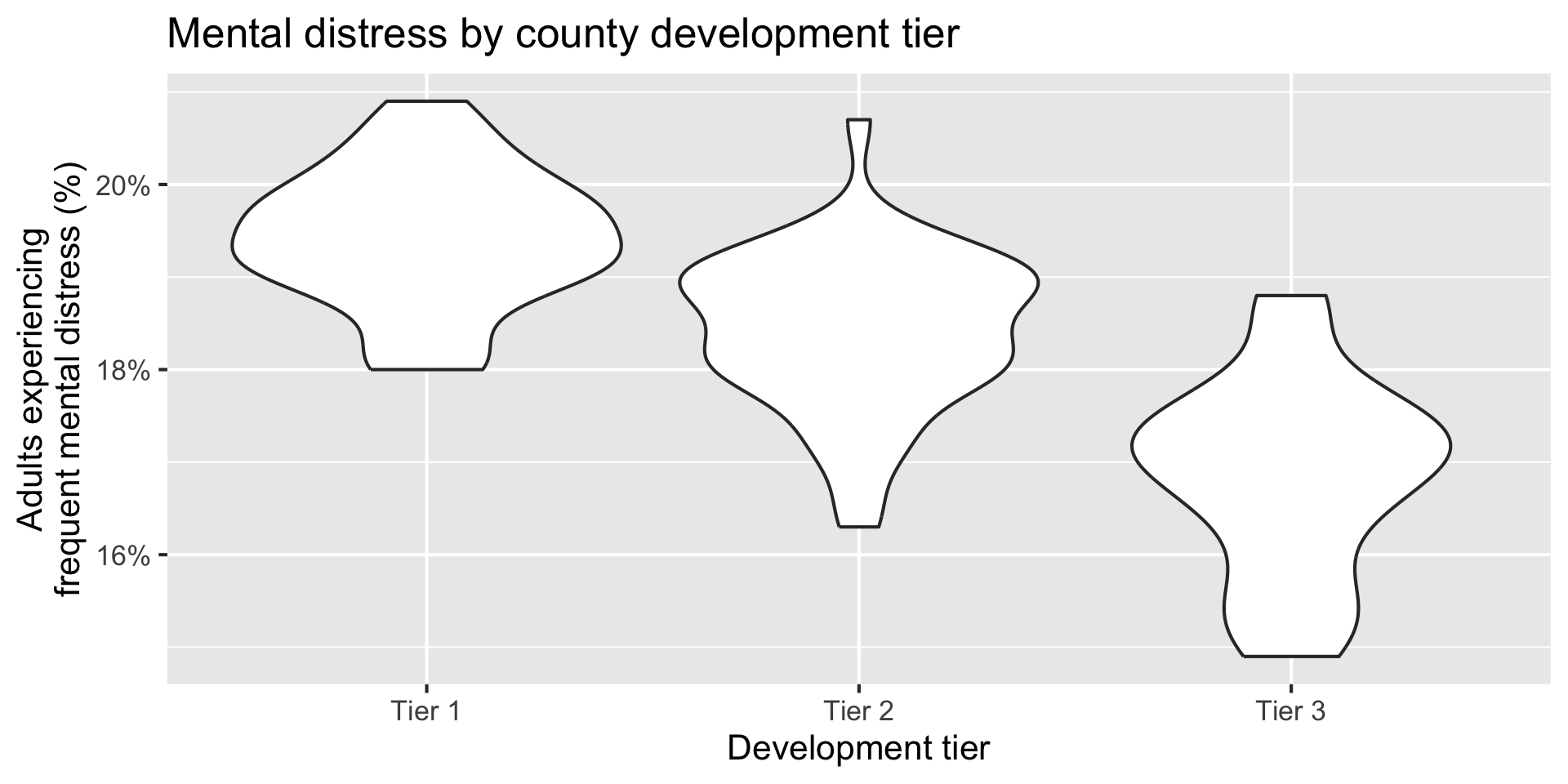
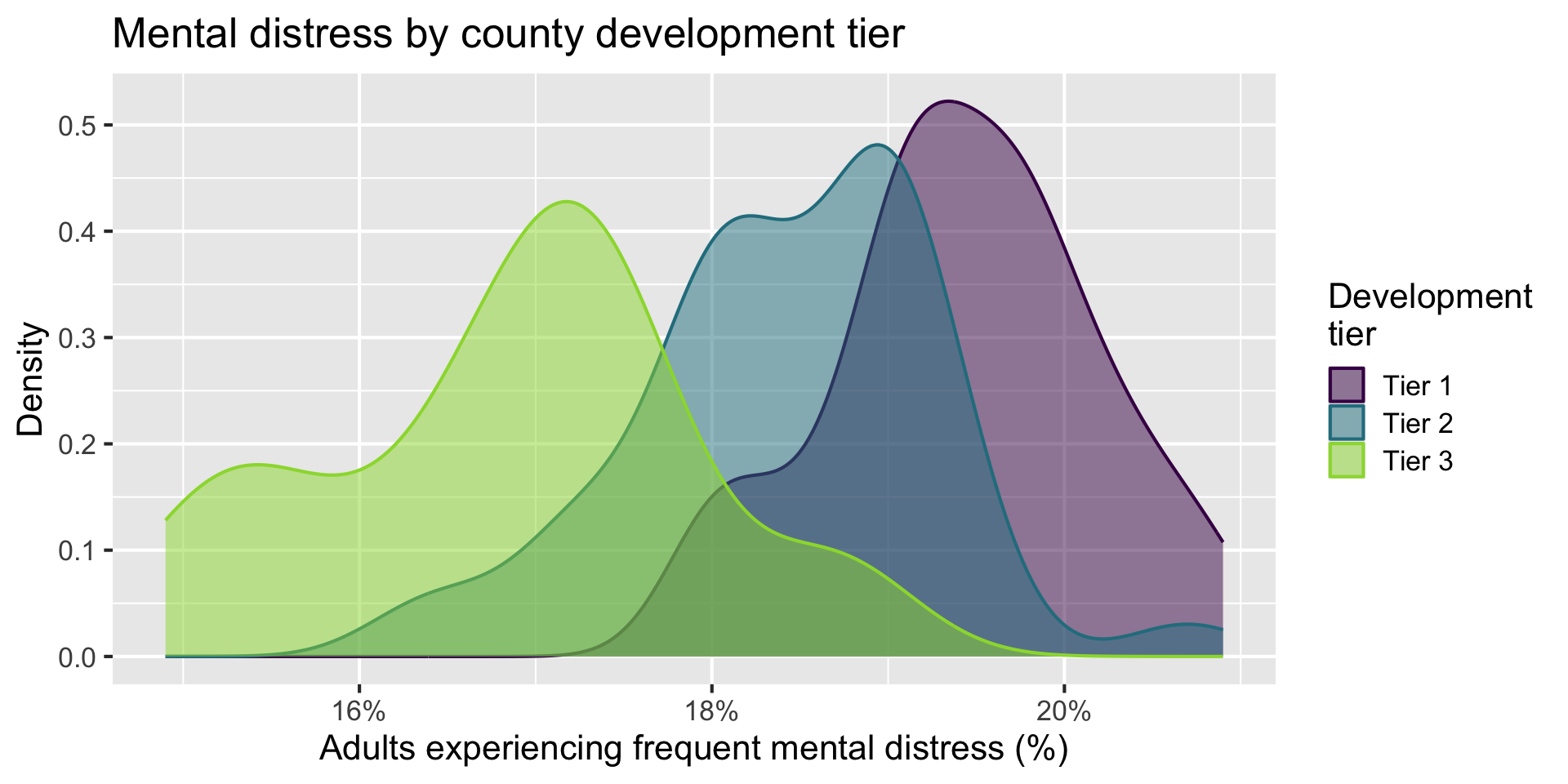
Determine whether each of the following plot types would be an appropriate choice for visualizing the relationship between mental-distress prevalence and development tier.
Scatterplot ❌
Box plot ✅
Violin plot ✅
Density plot ✅
Bar plot ❌
Stacked bar plot ❌
Boxplot
Code
ggplot(nc_places,aes(x =development_tier, y =mental_distress))+geom_boxplot()+scale_y_continuous(labels =label_percent(scale =1))+labs( x ="Development tier", y ="Adults experiencing\nfrequent mental distress (%)", title ="Mental distress by county development tier")
Violin plot
Code
ggplot(nc_places,aes(x =development_tier, y =mental_distress))+geom_violin()+scale_y_continuous(labels =label_percent(scale =1))+labs( x ="Development tier", y ="Adults experiencing\nfrequent mental distress (%)", title ="Mental distress by county development tier")
Density plot
Code
ggplot(nc_places,aes( x =mental_distress, color =development_tier, fill =development_tier))+geom_density(alpha =0.5)+scale_x_continuous(labels =label_percent(scale =1))+scale_color_viridis_d(end =0.85)+scale_fill_viridis_d(end =0.85)+labs( x ="Adults experiencing frequent mental distress (%)", y ="Density", color ="Development\ntier", fill ="Development\ntier", title ="Mental distress by county development tier")
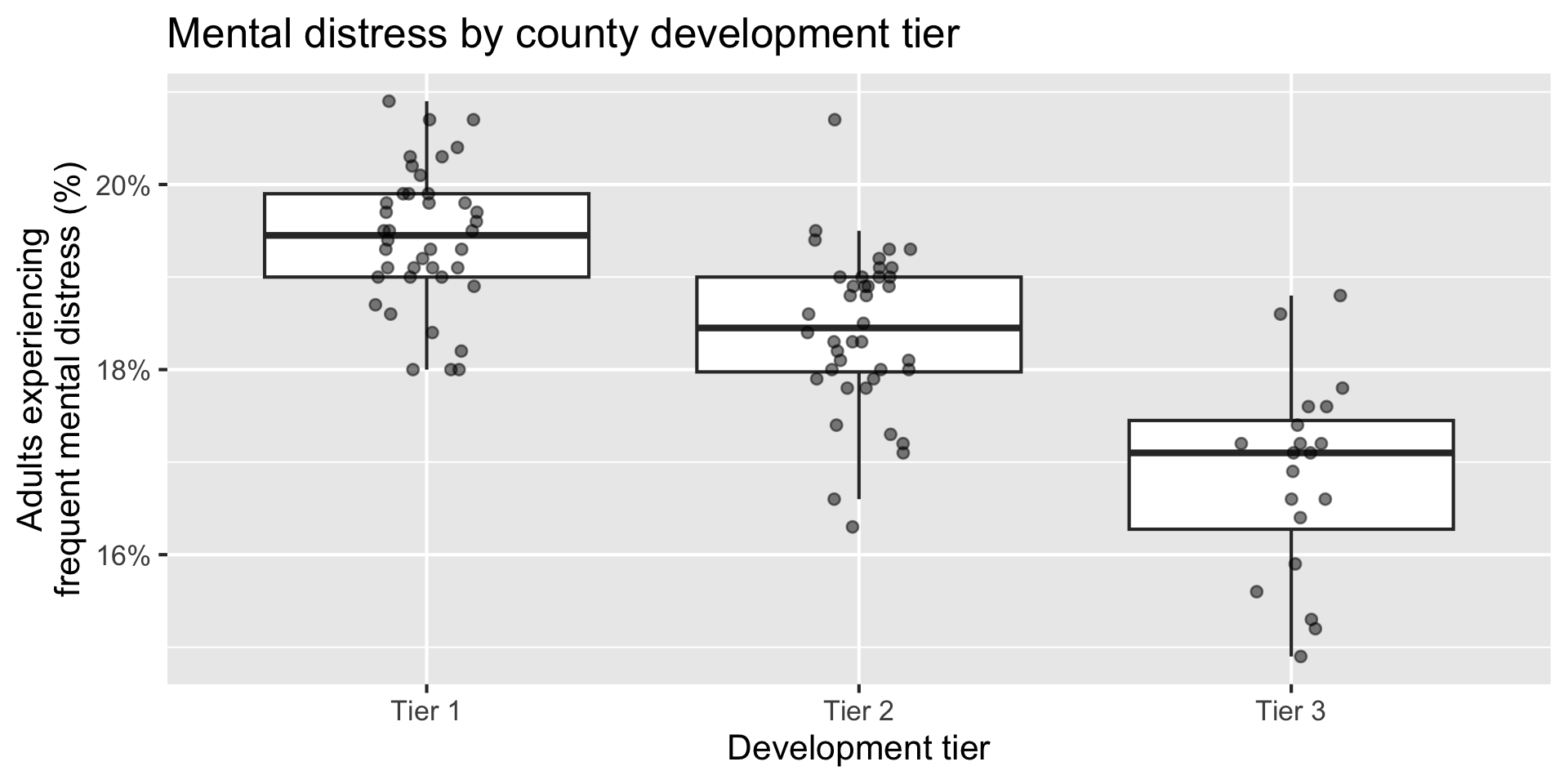
Multiple geoms
Code
ggplot(nc_places,aes(x =development_tier, y =mental_distress))+geom_boxplot(outlier.shape =NA)+geom_jitter(width =0.12, height =0, size =2, alpha =0.5)+scale_y_continuous(labels =label_percent(scale =1))+labs( x ="Development tier", y ="Adults experiencing\nfrequent mental distress (%)", title ="Mental distress by county development tier")
Summarize
Calculate the average mental-distress prevalence for counties in each development tier. How do the averages compare across tiers?
The predicted average mental-distress prevalence among Tier 1 counties is 19.4%.
Model - predict
What is the predicted mental-distress prevalence for a Tier 1 county? What are the predicted values for Tier 2 and Tier 3 counties? Where have we seen these values before?
A categorical predictor is encoded using dummy variables. A predictor with \(k\) levels requires \(k - 1\) dummy variables.
The first level of the categorical variable is the baseline level. In a model with one categorical predictor, the intercept is the predicted value of the outcome for the baseline level (when all dummy variables equal 0).
Each slope coefficient describes the difference between the predicted value of the outcome for that level of the categorical variable compared to the baseline level.
Changing the baseline level
By default, R uses the first level of a categorical variable as the baseline level.
We can change the baseline level by reordering the levels of the categorical variable.
Participate 📱💻
What function goes in the blank to make Tier 3 the baseline level in the development_tier variable?